2.8 Graphical Analysis of One-Dimensional Motion

Learning Objectives

By the end of this section, you will be able to:

Describe a straight-line graph in terms of its slope and y-intercept.
Determine average velocity or instantaneous velocity from a graph of position vs. time.
Determine average or instantaneous acceleration from a graph of velocity vs. time.
Derive a graph of velocity vs. time from a graph of position vs. time.
Derive a graph of acceleration vs. time from a graph of velocity vs. time.

A graph, like a picture, is worth a thousand words. Graphs not only contain numerical information; they also reveal relationships between physical quantities. This section uses graphs of position, velocity, and acceleration versus time to illustrate one-dimensional kinematics.

Slopes and General Relationships

First note that graphs in this text have perpendicular axes, one horizontal and the other vertical. When two physical quantities are plotted against one another in such a graph, the horizontal axis is usually considered to be an independent variable and the vertical axis a dependent variable. If we call the horizontal axis the $x$ -axis and the vertical axis the $y$ -axis, as in Figure 2.46, a straight-line graph has the general form

$y = mx + b .$

Here $m$ is the slope, defined to be the rise divided by the run (as seen in the figure) of the straight line. The letter $b$ is used for the y-intercept, which is the point at which the line crosses the vertical axis.

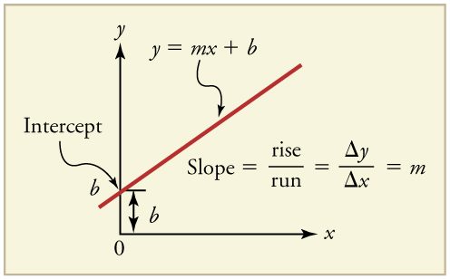
Graph of a straight-line sloping up at about 40 degrees. — **Figure 2.46** A straight-line graph. The equation for a straight line is $y = mx + b$ .

Graph of Position vs. Time (a = 0, so v is constant)

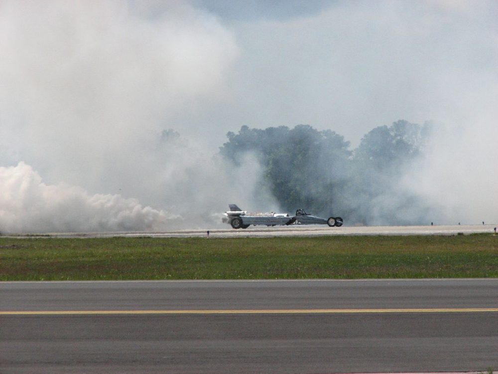
Time is usually an independent variable that other quantities, such as position, depend upon. A graph of position versus time would, thus, have $x$ on the vertical axis and $t$ on the horizontal axis. Figure 2.47 is just such a straight-line graph. It shows a graph of position versus time for a jet-powered car on a very flat dry lake bed in Nevada.

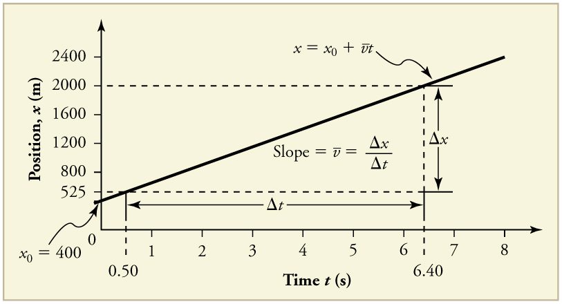
Line graph of jet car displacement in meters versus time in seconds. The line is straight with a positive slope. The y intercept is four hundred meters. The total change in time is eight point zero seconds. The initial position is four hundred meters. The final position is two thousand meters. — **Figure 2.47** Graph of position versus time for a jet-powered car on the Bonneville Salt Flats.

Using the relationship between dependent and independent variables, we see that the slope in the graph above is average velocity $\bar{v}$ and the intercept is position at time zero—that is, $x sub 0$ . Substituting these symbols into $y = mx + b$ gives

$x = \bar{v} t + x_{0}$

$x = x_{0} + \bar{v} t .$

Thus a graph of position versus time gives a general relationship among displacement(change in position), velocity, and time, as well as giving detailed numerical information about a specific situation.

From the figure we can see that the car has a position of 525 m at 0.50 s and 2000 m at 6.40 s. Its position at other times can be read from the graph; furthermore, information about its velocity and acceleration can also be obtained from the graph.

Example 1 Determining Average Velocity from a Graph of Position versus Time: Jet Car

Find the average velocity of the car whose position is graphed in Figure 2.47.

Strategy

The slope of a graph of $x$ vs. $t$ is average velocity, since slope equals rise over run. In this case, rise = change in position and run = change in time, so that

$slope = \frac{Δ x}{Δ t} = \bar{v} .$

Since the slope is constant here, any two points on the graph can be used to find the slope. (Generally speaking, it is most accurate to use two widely separated points on the straight line. This is because any error in reading data from the graph is proportionally smaller if the interval is larger.)

Solution

1. Choose two points on the line. In this case, we choose the points labeled on the graph: (6.4 s, 2000 m) and (0.50 s, 525 m). (Note, however, that you could choose any two points.)

2. Substitute the $x$ and $t$ values of the chosen points into the equation. Remember in calculating change $(Δ)$ we always use final value minus initial value.

$\bar{v} = \frac{Δ x}{Δ t} = \frac{2000 m - 525 m}{6 . 4 s - 0 . 50 s},$

yielding

$\bar{v} = 250 m/s .$

Discussion

This is an impressively large land speed (900 km/h, or about 560 mi/h): much greater than the typical highway speed limit of 60 mi/h (27 m/s or 96 km/h), but considerably shy of the record of 343 m/s (1234 km/h or 766 mi/h) set in 1997.

Graphs of Motion when $a$ is constant but $a not equal to 0$

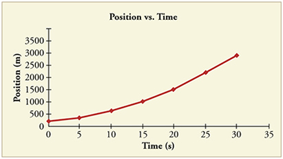
The graphs in Figure 2.48 below represent the motion of the jet-powered car as it accelerates toward its top speed, but only during the time when its acceleration is constant. Time starts at zero for this motion (as if measured with a stopwatch), and the position and velocity are initially 200 m and 15 m/s, respectively.

Three line graphs. First is a line graph of displacement over time. Line has a positive slope that increases with time. Second line graph is of velocity over time. Line is straight with a positive slope. Third line graph is of acceleration over time. Line is straight and horizontal, indicating constant acceleration. — **Figure 2.48** Graphs of motion of a jet-powered car during the time span when its acceleration is constant. (a) The slope of an $x$ vs. $t$ graph is velocity. This is shown at two points, and the instantaneous velocities obtained are plotted in the next graph. Instantaneous velocity at any point is the slope of the tangent at that point. (b) The slope of the $v$ vs. $t$ graph is constant for this part of the motion, indicating constant acceleration. (c) Acceleration has the constant value of $5. 0 m/s squared$ over the time interval plotted.

A photo shows a U S Air Force jet speeding down a track with a lot of smoke around it. — **Figure 2.49** A U.S. Air Force jet car speeds down a track.A U.S. Air Force jet car speeds down a track. (credit: Matt Trostle, Flickr)

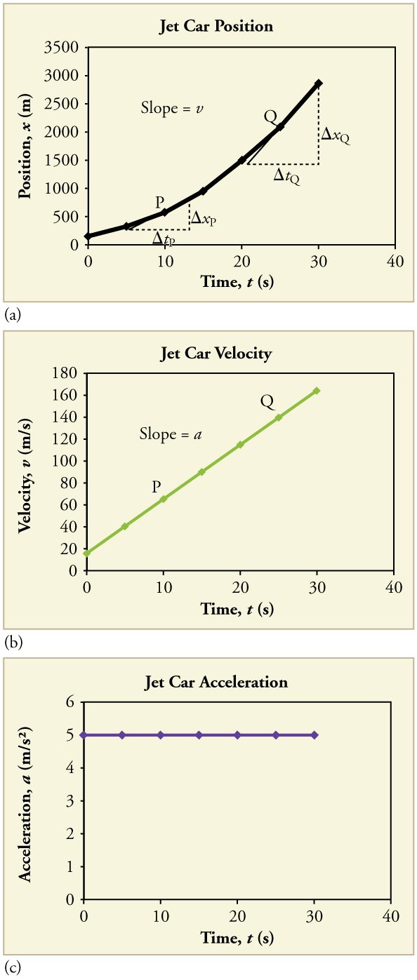
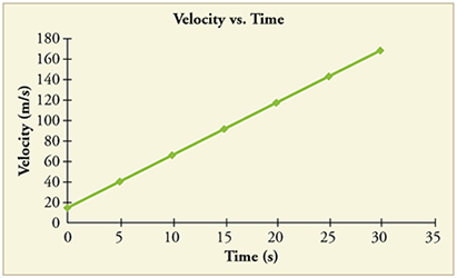
The graph of position versus time in Figure 2.48(a) is a curve rather than a straight line. The slope of the curve becomes steeper as time progresses, showing that the velocity is increasing over time. The slope at any point on a position-versus-time graph is the instantaneous velocity at that point. It is found by drawing a straight line tangent to the curve at the point of interest and taking the slope of this straight line. Tangent lines are shown for two points in Figure 2.48(a). If this is done at every point on the curve and the values are plotted against time, then the graph of velocity versus time shown in Figure 2.48(b) is obtained. Furthermore, the slope of the graph of velocity versus time is acceleration, which is shown in Figure 2.48(c).

Example 2 Determining Instantaneous Velocity from the Slope at a Point: Jet Car

Calculate the velocity of the jet car at a time of 25 s by finding the slope of the $x$ vs. $t$ graph in the graph below.

Figure 2.50 The slope of an

x

vs.

t

graph is velocity. This is shown at two points. Instantaneous velocity at any point is the slope of the tangent at that point.

Strategy

The slope of a curve at a point is equal to the slope of a straight line tangent to the curve at that point. This principle is illustrated in Figure 2.50, where Q is the point at $t equals 25 s$ .

Solution

1. Find the tangent line to the curve at $t equals 25 s$ .

2. Determine the endpoints of the tangent. These correspond to a position of 1300 m at time 19 s and a position of 3120 m at time 32 s.

3. Plug these endpoints into the equation to solve for the slope, $v$ .

$slope = v_{Q} = \frac{{Δ x}_{Q}}{{Δ t}_{Q}} = \frac{(3120 m - 1300 m)}{(32 s - 19 s)}$

Thus,

$v_{Q} = \frac{1820 m}{13 s} = 140 m/s.$

Discussion

This is the value given in this figure’s table for $v$ at $t equals 25 s$ . The value of 140 m/s for $v_{Q}$ is plotted in Figure 2.50. The entire graph of $v$ vs. $t$ can be obtained in this fashion.

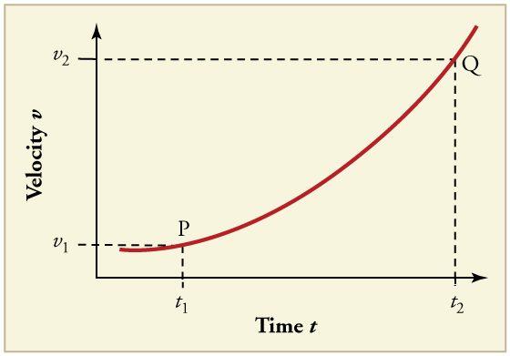
Carrying this one step further, we note that the slope of a velocity versus time graph is acceleration. Slope is rise divided by run; on a $v$ vs. $t$ graph, rise = change in velocity $Δ v$ and run = change in time $Δ t$ .

Since the velocity versus time graph in Figure 2.48(b) is a straight line, its slope is the same everywhere, implying that acceleration is constant. Acceleration versus time is graphed in Figure 2.48(c).

Additional general information can be obtained from Figure 2.50 and the expression for a straight line, $y = mx + b$ .

In this case, the vertical axis $y$ is $V$ , the intercept $b$ is $v sub 0$ , the slope $m$ is $a$ , and the horizontal axis $x$ is $t$ . Substituting these symbols yields

$v = v_{0} + at .$

A general relationship for velocity, acceleration, and time has again been obtained from a graph. Notice that this equation was also derived algebraically from other motion equations in Motion Equations for Constant Acceleration in One Dimension.

It is not accidental that the same equations are obtained by graphical analysis as by algebraic techniques. In fact, an important way to discover physical relationships is to measure various physical quantities and then make graphs of one quantity against another to see if they are correlated in any way. Correlations imply physical relationships and might be shown by smooth graphs such as those above. From such graphs, mathematical relationships can sometimes be postulated. Further experiments are then performed to determine the validity of the hypothesized relationships.

Graphs of Motion Where Acceleration is Not Constant

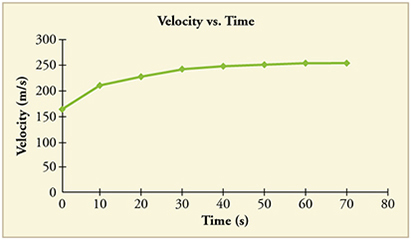
Now consider the motion of the jet car as it goes from 165 m/s to its top velocity of 250 m/s, graphed in Figure 2.51. Time again starts at zero, and the initial velocity is 165 m/s. (This was the final velocity of the car in the motion graphed in Figure 2.48.) Acceleration gradually decreases from $5. 0 m/s squared$ to zero when the car hits 250 m/s. The velocity increases until 55 s and then becomes constant, since acceleration decreases to zero at 55 s and remains zero afterward.

Two line graphs of jet car velocity and acceleration, respectively. First line graph is of velocity over time. Line graph has a positive slope that decreases over time and flattens out at the end. Second line graph is of acceleration over time. Line has a negative slope that increases over time until it flattens out at the end. The line is not smooth, but has several kinks. — **Figure 2.51** Graphs of motion of a jet-powered car as it reaches its top velocity. This motion begins where the motion in Figure 2.48 ends. (a) The velocity gradually approaches its top value. The slope of this graph is acceleration. It is plotted in the final graph. (b) Acceleration gradually declines to zero when velocity becomes constant. Notice in each of the three graphs that the acceleration drops down to zero and the velocity levels out. This results in a position-time graph that is almost linear. A close-up of the position time graph would show a slight curvature, as indicated in the velocity graph.

Example 3 Calculating Acceleration from a Graph of Velocity versus Time

Calculate the acceleration of the jet car at a time of 25 s by finding the slope of the $v$ vs. $t$ graph in Figure 2.51(a).

Strategy

The slope of the curve at $t equals 25 s$ is equal to the slope of the line tangent at that point, as illustrated in Figure 2.51(a).

Solution

Determine endpoints of the tangent line from the figure, and then plug them into the equation to solve for slope, $a$ .

$slope = \frac{Δ v}{Δ t} = \frac{(260 m/s - 210 m/s)}{(51 s - 1.0 s)}$

$a = \frac{50 m/s}{50 s} = 1 . 0 m {/s}^{2} .$

Discussion

Note that this value for $a$ is consistent with the value plotted in Figure 2.51(b) at $t equals 25 s$ .

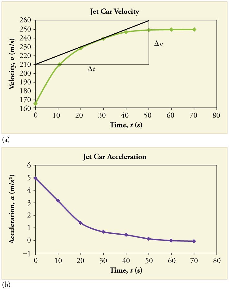
A graph of position versus time can be used to generate a graph of velocity versus time, and a graph of velocity versus time can be used to generate a graph of acceleration versus time. We do this by finding the slope of the graphs at every point. If the graph is linear (i.e., a line with a constant slope), it is easy to find the slope at any point and you have the slope for every point. Graphical analysis of motion can be used to describe both specific and general characteristics of kinematics. Graphs can also be used for other topics in physics. An important aspect of exploring physical relationships is to graph them and look for underlying relationships.

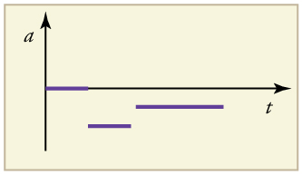
A graph of velocity vs. time of a ship coming into a harbor is shown below. (a) Describe the motion of the ship based on the graph. (b)What would a graph of the ship’s acceleration look like?

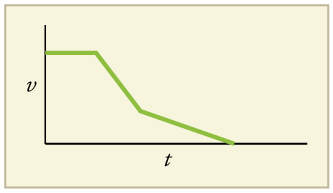
Line graph of velocity versus time. The line has three legs. The first leg is flat. The second leg has a negative slope. The third leg also has a negative slope, but the slope is not as negative as the second leg. — **Figure 2.52**

(a) The ship moves at constant velocity and then begins to decelerate at a constant rate. At some point, its deceleration rate decreases. It maintains this lower deceleration rate until it stops moving.

(b) A graph of acceleration vs. time would show zero acceleration in the first leg, large and constant negative acceleration in the second leg, and constant negative acceleration.

A line graph of acceleration versus time. There are three legs of the graph. All three legs are flat and straight. The first leg shows constant acceleration of 0. The second leg shows a constant negative acceleration. The third leg shows a constant negative acceleration that is not as negative as the second leg. — **Figure 2.53**

Section Summary

Graphs of motion can be used to analyze motion.
Graphical solutions yield identical solutions to mathematical methods for deriving motion equations.
The slope of a graph of displacement $x$ vs. time $t$ is velocity $v$ .
The slope of a graph of velocity $v$ vs. time $t$ graph is acceleration $a$ .
Average velocity, instantaneous velocity, and acceleration can all be obtained by analyzing graphs.

Conceptual Questions

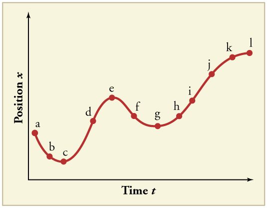
(a) Explain how you can use the graph of position versus time in Figure 2.54 to describe the change in velocity over time. Identify (b) the time ( $t_{a}$ , $t_{b}$ , $t_{c}$ , $t_{d}$ , or $t_{e}$ ) at which the instantaneous velocity is greatest, (c) the time at which it is zero, and (d) the time at which it is negative.

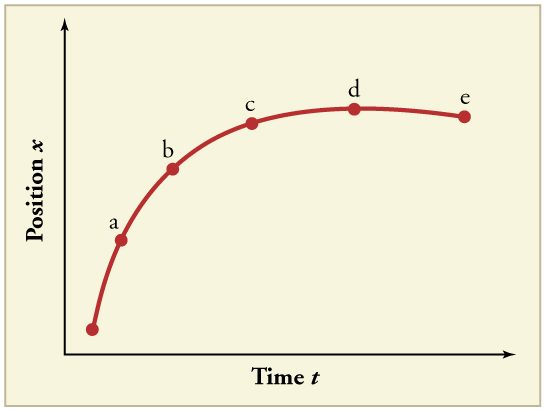
Line graph of position versus time with 5 points labeled: a, b, c, d, and e. The slope of the line changes. It begins with a positive slope that decreases over time until around point d, where it is flat. It then has a slightly negative slope. — **Figure 2.54**

(a) Sketch a graph of velocity versus time corresponding to the graph of position versus time given in Figure 2.55. (b) Identify the time or times ( $t_{a}$ , $t_{b}$ , $t_{c}$ , etc.) at which the instantaneous velocity is greatest. (c) At which times is it zero? (d) At which times is it negative?

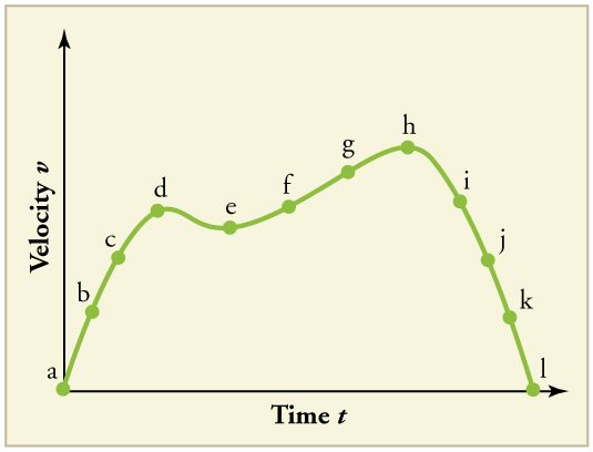
Line graph of position over time with 12 points labeled a through l. Line has a negative slope from a to c, where it turns and has a positive slope till point e. It turns again and has a negative slope till point g. The slope then increases again till l, where it flattens out. — **Figure 2.55**

(a) Explain how you can determine the acceleration over time from a velocity versus time graph such as the one in Figure 2.56. (b) Based on the graph, how does acceleration change over time?

Line graph of velocity over time with two points labeled. Point P is at v 1 t 1. Point Q is at v 2 t 2. The line has a positive slope that increases over time. — **Figure 2.56**

(a) Sketch a graph of acceleration versus time corresponding to the graph of velocity versus time given in Figure 2.57. (b) Identify the time or times ( $t_{a}$ , $t_{b}$ , $t_{c}$ , etc.) at which the acceleration is greatest. (c) At which times is it zero? (d) At which times is it negative?

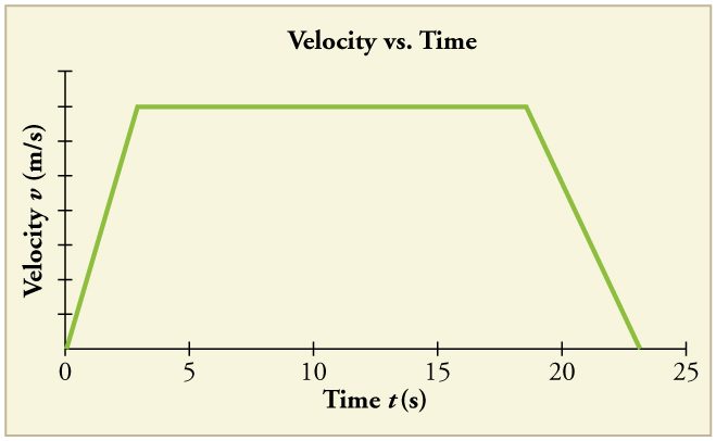
Line graph of velocity over time with 12 points labeled a through l. The line has a positive slope from a at the origin to d where it slopes downward to e, and then back upward to h. It then slopes back down to point l at v equals 0. — **Figure 2.57**

Consider the velocity vs. time graph of a person in an elevator shown in Figure 2.58. Suppose the elevator is initially at rest. It then accelerates for 3 seconds, maintains that velocity for 15 seconds, then decelerates for 5 seconds until it stops. The acceleration for the entire trip is not constant so we cannot use the equations of motion from Motion Equations for Constant Acceleration in One Dimension for the complete trip. (We could, however, use them in the three individual sections where acceleration is a constant.) Sketch graphs of (a) position vs. time and (b) acceleration vs. time for this trip.

Line graph of velocity versus time. Line begins at the origin and has a positive slope until it reaches 3 meters per second at 3 seconds. The slope is then zero until 18 seconds, where it becomes negative until the line reaches a velocity of 0 at 23 seconds. — **Figure 2.58**

A cylinder is given a push and then rolls up an inclined plane. If the origin is the starting point, sketch the position, velocity, and acceleration of the cylinder vs. time as it goes up and then down the plane.

Problems & Exercises

Note: There is always uncertainty in numbers taken from graphs. If your answers differ from expected values, examine them to see if they are within data extraction uncertainties estimated by you.

(a) By taking the slope of the curve in Figure 2.59, verify that the velocity of the jet car is 115 m/s at $t equals 20 s$ . (b) By taking the slope of the curve at any point in Figure 2.60, verify that the jet car’s acceleration is $5. 0 m/s squared$ .

Line graph of position over time. Line has positive slope that increases over time. — **Figure 2.59**

Line graph of velocity versus time. Line is straight with a positive slope. — **Figure 2.60**

(a) $115 m/s$

(b) $5. 0 m/s squared$

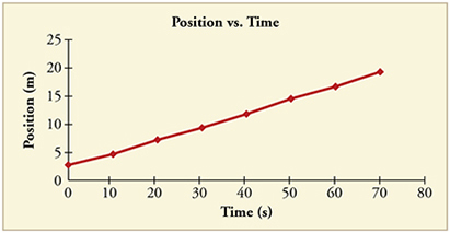
(a) Using approximate values, calculate the slope of the curve in Figure 2.61 to verify that the velocity at $t equals 10 s$ is approximately 0.21 m/s.

Using approximate values, calculate the slope of the curve in Figure 2.61 at $t equals 10.0 s$ and at $t equals 30 s$ find the velocity at these times. (b) Using your answer to part a, find the approximate acceleration at $t equals 20 s$ . Assume all values are known to 2 significant figures.

Line graph of position versus time. Line is straight with a positive slope. — **Figure 2.61**

$t equals 10$

By taking the slope of the curve in Figure 2.62, verify that the acceleration is $3. 2 m /s squared$ at $t equals 10 s$ .

Line graph of velocity versus time. Line has a positive slope that decreases over time until the line flattens out. — **Figure 2.62**

Construct the position graph for the subway shuttle train as shown in Figure 2.19(a). Your graph should show the position of the train, in kilometers, from t = 0 to 20 s. You will need to use the information on acceleration and velocity given in the examples for this figure.

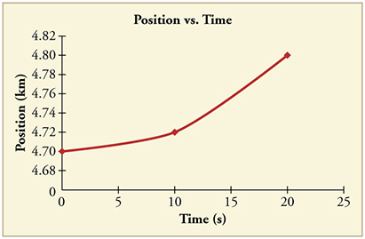
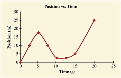
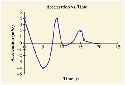
Line graph of position versus time. Line begins with a slight positive slope. It then kinks to a much greater positive slope.

(a) Take the slope of the curve in Figure 2.63 to find the jogger’s velocity at $t equals 2. 5 s$ . (b) Repeat at 7.5 s. These values must be consistent with the graph in Figure 2.64.

Line graph of position over time. Line begins sloping upward, then kinks back down, then kinks back upward again. — **Figure 2.63**

Line graph of velocity over time. Line begins with a positive slope, then kinks downward with a negative slope, then kinks back upward again. It kinks back down again slightly, then back up again, and ends with a slightly less positive slope. — **Figure 2.64**

Line graph of acceleration over time. Line begins with a negative slope, then curves upward with a positive slope, then kinks back upward again. It kinks back down again, then more gradually back up again, then curves back down again, and ends with a slightly negative slope. — **Figure 2.65**

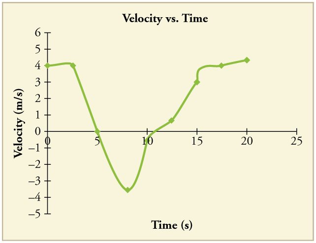
A graph of $v (t)$ is shown for a world-class track sprinter in a 100-m race. (See Figure 2.66). (a) What is his average velocity for the first 4 s? (b) What is his instantaneous velocity at $t equals 5 s$ ? (c) What is his average acceleration between 0 and 4 s? (d) What is his time for the race?

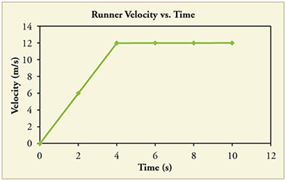
Line graph of velocity versus time. The line has two legs. The first has a constant positive slope. The second is flat, with a slope of 0. — **Figure 2.66**

(a) 6 m/s

(b) 12 m/s

(d) 10 s

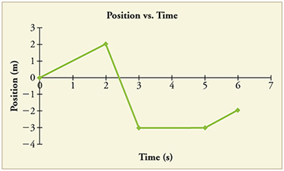
Figure 2.67 shows the position graph for a particle for 6 s. (a) Draw the corresponding Velocity vs. Time graph. (b) What is the acceleration between 0 s and 2 s? (c) What happens to the acceleration at exactly 2 s?

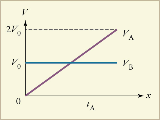
Line graph of position versus time. The line has 4 legs. The first leg has a positive slope. The second leg has a negative slope. The third has a slope of 0. The fourth has a positive slope. — **Figure 2.67**

Critical Thinking Two cars are side by side on a path where friction is negligible. Car A starts from rest and has a positive, constant acceleration while car B travels at a constant speed. The cars reach the same check point down the road at the same time. (a) Which car is traveling faster at the check point? Briefly explain your reasoning. (b) Based on experimental data, an equation that fits the data is suggested for the speed of car A at the check point, V, which may not be correct: $V equals K V sub 0$ , where K is a constant with appropriate units and $V sub 0$ is the initial velocity of car B. Is this equation consistent with your answer from part a? Explain why or why not. Does this equation make sense? Explain why or why not. (c) Graph the velocity of car A and the velocity of car B vs. distance along the path, starting when the cars are side by side.

(a) Car A is traveling faster at the checkpoint because it must go past the speed of car B to reach the same distance.

(b) i. Yes, the equation is consistent with the answer because the speed of car A is only a constant away from the correct answer. ii. Yes, the equation makes sense because $V equals 2 V sub 0$ .

(c)

The figure shows velocity v graphed as a function of position x. The plot of V sub A is linear, with a positive slope, starting at the origin and ending at a maximum velocity of 2 times v sub 0 at velocity v sub zero. The plot of V sub B is a constant at velocity v sub zero. — **Figure 2.68**

Adapted from College Physics 2e by OpenStax (openstax.org), licensed under CC BY-NC-SA 4.0. Changes were made. License: CC-BY-NC-SA-4.0.

2.8 Graphical Analysis of One-Dimensional Motion

Learning Objectives

Slopes and General Relationships

Graph of Position vs. Time (a = 0, so v is constant)

Graphs of Motion when a is constant but a≠0

Graphs of Motion Where Acceleration is Not Constant

Section Summary

Conceptual Questions

Problems & Exercises

Graphs of Motion when $a$ is constant but $a not equal to 0$