2.4 Acceleration

Learning Objectives

By the end of this section, you will be able to:

Define and distinguish between instantaneous acceleration, average acceleration, and deceleration.
Calculate acceleration given initial time, initial velocity, final time, and final velocity.

An airplane flying very low to the ground, just above a beach full of onlookers, as it comes in for a landing. — **Figure 2.13** A plane decelerates, or slows down, as it comes in for landing in St. Maarten. Its acceleration is opposite in direction to its velocity.A plane decelerates, or slows down, as it comes in for landing in St. Maarten. Its acceleration is opposite in direction to its velocity. (credit: Steve Conry, Flickr)

In everyday conversation, to accelerate means to speed up. The accelerator in a car can in fact cause it to speed up. The greater the acceleration, the greater the change in velocity over a given time. The formal definition of acceleration is consistent with these notions, but more inclusive.

Because acceleration is velocity in m/s divided by time in s, the SI units for acceleration are $m/s squared$ , meters per second squared or meters per second per second, which literally means by how many meters per second the velocity changes every second.

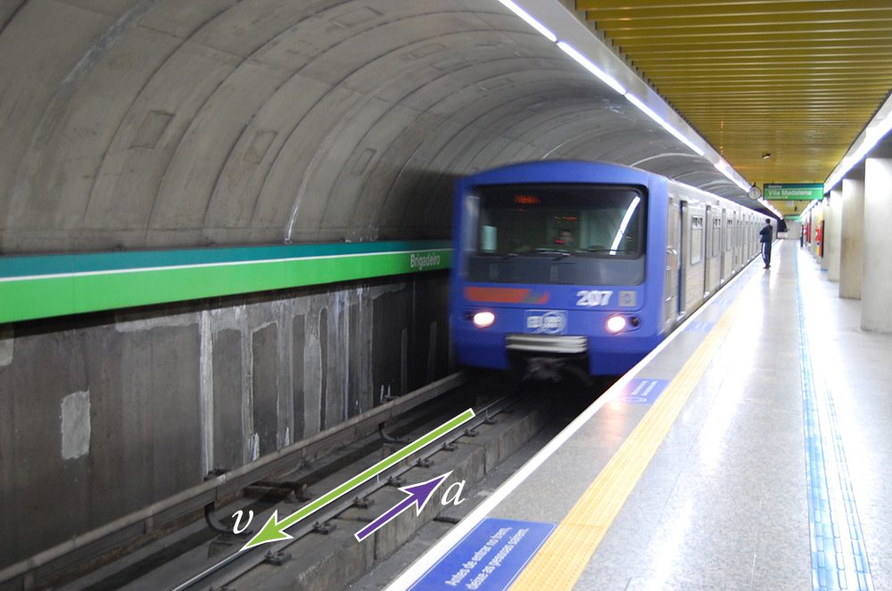
Recall that velocity is a vector—it has both magnitude and direction. This means that a change in velocity can be a change in magnitude (or speed), but it can also be a change in direction. For example, if a car turns a corner at constant speed, it is accelerating because its direction is changing. The quicker you turn, the greater the acceleration. So there is an acceleration when velocity changes either in magnitude (an increase or decrease in speed) or in direction, or both.

Keep in mind that although acceleration is in the direction of the change in velocity, it is not always in the direction of motion. When an object slows down, its acceleration is opposite to the direction of its motion. This is known as deceleration.

A subway train arriving at a station. A velocity vector arrow points along the track away from the train. An acceleration vector arrow points along the track toward the train. — **Figure 2.14** A subway train in Sao Paulo, Brazil, decelerates as it comes into a station. It is accelerating in a direction opposite to its direction of motion.A subway train in Sao Paulo, Brazil, decelerates as it comes into a station. It is accelerating in a direction opposite to its direction of motion. (credit: Yusuke Kawasaki, Flickr)

Note

Misconception Alert: Deceleration vs. Negative Acceleration

Deceleration always refers to acceleration in the direction opposite to the direction of the velocity. Deceleration always reduces speed. Negative acceleration, however, is acceleration in the negative direction in the chosen coordinate system. Negative acceleration may or may not be deceleration, and deceleration may or may not be considered negative acceleration. For example, consider Figure 2.15.

Figure 2.15 (a) This car is speeding up as it moves toward the right. It therefore has positive acceleration in our coordinate system. (b) This car is slowing down as it moves toward the right. Therefore, it has negative acceleration in our coordinate system, because its acceleration is toward the left. The car is also decelerating: the direction of its acceleration is opposite to its direction of motion. (c) This car is moving toward the left, but slowing down over time. Therefore, its acceleration is positive in our coordinate system because it is toward the right. However, the car is decelerating because its acceleration is opposite to its motion. (d) This car is speeding up as it moves toward the left. It has negative acceleration because it is accelerating toward the left. However, because its acceleration is in the same direction as its motion, it is speeding up (not decelerating).

Example 1 Calculating Acceleration: A Racehorse Leaves the Gate

A racehorse coming out of the gate accelerates from rest to a velocity of 15.0 m/s due west in 1.80 s. What is its average acceleration?

Figure 2.16 (credit: Jon Sullivan, PD Photo.org)

Strategy

First we draw a sketch and assign a coordinate system to the problem. This is a simple problem, but it always helps to visualize it. Notice that we assign east as positive and west as negative. Thus, in this case, we have negative velocity.

Figure 2.17

We can solve this problem by identifying $Δ v$ and $Δ t$ from the given information and then calculating the average acceleration directly from the equation $\bar{a} = \frac{Δ v}{Δ t} = \frac{v_{f} - v_{0}}{t_{f} - t_{0}}$ .

Solution

1. Identify the knowns. $v sub 0 equals 0$ , $v_{f} = - 15 .0 m/s$ (the negative sign indicates direction toward the west), $Δ t equals 1.80 s$ .

2. Find the change in velocity. Since the horse is going from zero to $minus 15.0 m/s$ , its change in velocity equals its final velocity: $Δ v = v_{f} = - 15 .0 m/s$ .

3. Plug in the known values ( $Δ v$ and $Δ t$ ) and solve for the unknown $\bar{a}$ .

$\bar{a} = \frac{Δ v}{Δ t} = \frac{- 15 .0 m/s}{1 .80 s} = - 8 .33 m {/s}^{2} .$

Discussion

The negative sign for acceleration indicates that acceleration is toward the west. An acceleration of $8.33 m /s squared$ due west means that the horse increases its velocity by 8.33 m/s due west each second, that is, 8.33 meters per second per second, which we write as $8.33 m /s squared$ . This is truly an average acceleration, because the ride is not smooth. We shall see later that an acceleration of this magnitude would require the rider to hang on with a force nearly equal to his weight.

Instantaneous Acceleration

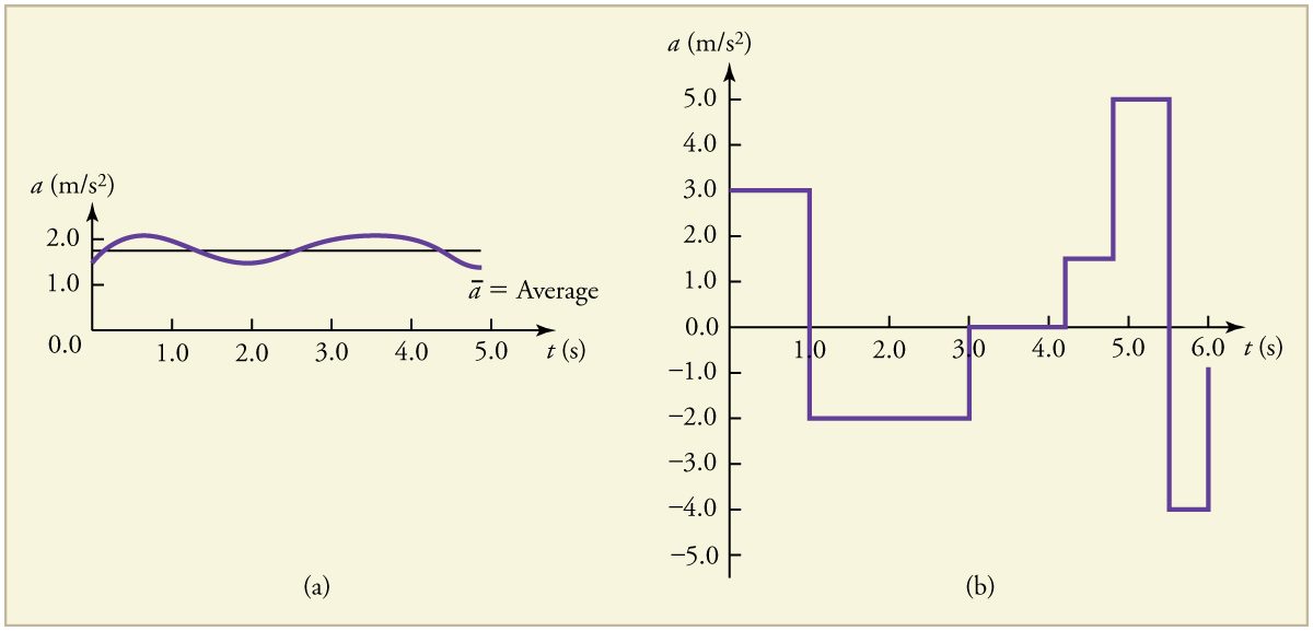
Instantaneous acceleration $a$ , or the acceleration at a specific instant in time, is obtained by the same process as discussed for instantaneous velocity in Time, Velocity, and Speed—that is, by considering an infinitesimally small interval of time. How do we find instantaneous acceleration using only algebra? The answer is that we choose an average acceleration that is representative of the motion. Figure 2.18 shows graphs of instantaneous acceleration versus time for two very different motions. In Figure 2.18(a), the acceleration varies slightly and the average over the entire interval is nearly the same as the instantaneous acceleration at any time. In this case, we should treat this motion as if it had a constant acceleration equal to the average (in this case about $1. 8 m /s squared$ ). In Figure 2.18(b), the acceleration varies drastically over time. In such situations it is best to consider smaller time intervals and choose an average acceleration for each. For example, we could consider motion over the time intervals from 0 to 1.0 s and from 1.0 to 3.0 s as separate motions with accelerations of $plus 3. 0 m /s squared$ and $–2. 0 m /s squared$ , respectively.

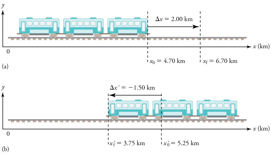
The next several examples consider the motion of the subway train shown in Figure 2.19. In (a) the shuttle moves to the right, and in (b) it moves to the left. The examples are designed to further illustrate aspects of motion and to illustrate some of the reasoning that goes into solving problems.

In part (a), a subway train moves from left to right from an initial position of x equals 4 point 7 kilometers to a final position of x equals 6 point 7 kilometers, with a displacement of 2 point 0 kilometers. In part (b), the train moves toward the left, from an initial position of 5 point 25 kilometers to a final position of 3 point 75 kilometers. — **Figure 2.19** One-dimensional motion of a subway train considered in Example 2, Example 3, Example 4, Example 5, Example 6, and Example 7. Here we have chosen the $x$ -axis so that + means to the right and $-$ means to the left for displacements, velocities, and accelerations. (a) The subway train moves to the right from $x sub 0$ to $x_{f}$ . Its displacement $Δ x$ is +2.0 km. (b) The train moves to the left from $x ′ sub 0$ to ${x'}_{f}$ . Its displacement $Δ x'$ is $minus 1.5 km$ . (Note that the prime symbol (′) is used simply to distinguish between displacement in the two different situations. The distances of travel and the size of the cars are on different scales to fit everything into the diagram.)

Example 2 Calculating Displacement: A Subway Train

What are the magnitude and sign of displacements for the motions of the subway train shown in parts (a) and (b) of Figure 2.19?

Strategy

A drawing with a coordinate system is already provided, so we don’t need to make a sketch, but we should analyze it to make sure we understand what it is showing. Pay particular attention to the coordinate system. To find displacement, we use the equation $Δ x = x_{f} - x_{0}$ . This is straightforward since the initial and final positions are given.

Solution

1. Identify the knowns. In the figure we see that $x sub f equals 6.70 km$ and $x sub 0 equals 4.70 km$ for part (a), and $x ′ sub f equals 3.75 km$ and $x ′ sub 0 equals 5.25 km$ for part (b).

2. Solve for displacement in part (a).

$Δ x = x_{f} - x_{0} = 6 . 70 km - 4 . 70 km = + 2 . 00 km$

3. Solve for displacement in part (b).

$Δ x' = {x'}_{f} - {x'}_{0} = 3.75 km - 5.25 km = - 1.50 km$

Discussion

The direction of the motion in (a) is to the right and therefore its displacement has a positive sign, whereas motion in (b) is to the left and thus has a negative sign.

Example 3 Comparing Distance Traveled with Displacement: A Subway Train

What are the distances traveled for the motions shown in parts (a) and (b) of the subway train in Figure 2.19?

Strategy

To answer this question, think about the definitions of distance and distance traveled, and how they are related to displacement. Distance between two positions is defined to be the magnitude of displacement, which was found in Example 2. Distance traveled is the total length of the path traveled between the two positions. (See Displacement.) In the case of the subway train shown in Figure 2.19, the distance traveled is the same as the distance between the initial and final positions of the train.

Solution

1. The displacement for part (a) was +2.00 km. Therefore, the distance between the initial and final positions was 2.00 km, and the distance traveled was 2.00 km.

2. The displacement for part (b) was $−1.5 km.$ Therefore, the distance between the initial and final positions was 1.50 km, and the distance traveled was 1.50 km.

Discussion

Distance is a scalar. It has magnitude but no sign to indicate direction.

Example 4 Calculating Acceleration: A Subway Train Speeding Up

Suppose the train in Figure 2.19(a) accelerates from rest to 30.0 km/h in the first 20.0 s of its motion. What is its average acceleration during that time interval?

Strategy

It is worth it at this point to make a simple sketch:

Figure 2.20

This problem involves three steps. First we must determine the change in velocity, then we must determine the change in time, and finally we use these values to calculate the acceleration.

Solution

1. Identify the knowns. $v sub 0 equals 0$ (the trains starts at rest), $v sub f equals 30. 0 km/h$ , and $Δ t equals 20. 0 s$ .

2. Calculate $Δ v$ . Since the train starts from rest, its change in velocity is $Δ v = + 30.0 km/h$ , where the plus sign means velocity to the right.

3. Plug in known values and solve for the unknown, $\bar{a}$ .

$\bar{a} = \frac{Δ v}{Δ t} = \frac{+ 30.0 km/h}{20 . 0 s}$

4. Since the units are mixed (we have both hours and seconds for time), we need to convert everything into SI units of meters and seconds. (See Physical Quantities and Units for more guidance.)

$\bar{a} = (\frac{+ 30 km/h}{20.0 s}) (\frac{10^{3} m}{1 km}) (\frac{1 h}{3600 s}) = 0 . {417 m/s}^{2}$

Discussion

The plus sign means that acceleration is to the right. This is reasonable because the train starts from rest and ends up with a velocity to the right (also positive). So acceleration is in the same direction as the change in velocity, as is always the case.

Example 5 Calculate Acceleration: A Subway Train Slowing Down

Now suppose that at the end of its trip, the train in Figure 2.19(a) slows to a stop from a speed of 30.0 km/h in 8.00 s. What is its average acceleration while stopping?

Strategy

Figure 2.21

In this case, the train is decelerating and its acceleration is negative because it is toward the left. As in the previous example, we must find the change in velocity and the change in time and then solve for acceleration.

Solution

1. Identify the knowns. $v sub 0 equals 30.0 km/h$ , $v sub f equals 0 km/h$ (the train is stopped, so its velocity is 0), and $Δ t equals 8.00 s$ .

2. Solve for the change in velocity, $Δ v$ .

$Δ v = v_{f} - v_{0} = 0 - 30 . 0 km/h = - 30 .0 km/h$

3. Plug in the knowns, $Δ v$ and $Δ t$ , and solve for $\bar{a}$ .

$\bar{a} = \frac{Δ v}{Δ t} = \frac{- 30 . 0 km/h}{8 . 00 s}$

4. Convert the units to meters and seconds.

$\bar{a} = \frac{Δ v}{Δ t} = (\frac{- 30.0 km/h}{8.00 s}) (\frac{10^{3} m}{1 km}) (\frac{1 h}{3600 s}) = {−1.04 m/s}^{2} .$

Discussion

The minus sign indicates that acceleration is to the left. This sign is reasonable because the train initially has a positive velocity in this problem, and a negative acceleration would oppose the motion. Again, acceleration is in the same direction as the change in velocity, which is negative here. This acceleration can be called a deceleration because it has a direction opposite to the velocity.

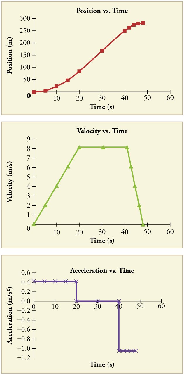
The graphs of position, velocity, and acceleration vs. time for the trains in Example 4 and Example 5 are displayed in Figure 2.22. (We have taken the velocity to remain constant from 20 to 40 s, after which the train decelerates.)

Three graphs. The first is a line graph of position in meters versus time in seconds. The line begins at the origin and has a concave up shape from time equals zero to time equals twenty seconds. It is straight with a positive slope from twenty seconds to forty seconds. It is then convex up from forty to fifty seconds. The second graph is a line graph of velocity in meters per second versus time in seconds. The line is straight with a positive slope beginning at the origin from 0 to twenty seconds. It is flat from twenty to forty seconds. From forty to fifty seconds the line is straight with a negative slope back down to a velocity of 0. The third graph is a line graph of acceleration in meters per second per second versus time in seconds. The line is flat with a positive constant acceleration from zero to twenty seconds. The line then drops to an acceleration of 0 from twenty to forty seconds. The line drops again to a negative acceleration from forty to fifty seconds. — **Figure 2.22** (a) Position of the train over time. Notice that the train’s position changes slowly at the beginning of the journey, then more and more quickly as it picks up speed. Its position then changes more slowly as it slows down at the end of the journey. In the middle of the journey, while the velocity remains constant, the position changes at a constant rate. (b) Velocity of the train over time. The train’s velocity increases as it accelerates at the beginning of the journey. It remains the same in the middle of the journey (where there is no acceleration). It decreases as the train decelerates at the end of the journey. (c) The acceleration of the train over time. The train has positive acceleration as it speeds up at the beginning of the journey. It has no acceleration as it travels at constant velocity in the middle of the journey. Its acceleration is negative as it slows down at the end of the journey.

Example 6 Calculating Average Velocity: The Subway Train

What is the average velocity of the train in part b of Example 2, and shown again below, if it takes 5.00 min to make its trip?

Figure 2.23

Strategy

Average velocity is displacement divided by time. It will be negative here, since the train moves to the left and has a negative displacement.

Solution

1. Identify the knowns. $x ′ sub f equals 3.75 km$ , $x ′ sub 0 equals 5.25 km$ , $Δ t equals 5.00 min$ .

2. Determine displacement, $Δ x'$ . We found $Δ x'$ to be $minus 1.5 km$ in Example 2.

3. Solve for average velocity.

$\bar{v} = \frac{Δ x'}{Δ t} = \frac{- 1.50 km}{5.00 min}$

4. Convert units.

$\bar{v} = \frac{Δ x'}{Δ t} = (\frac{- 1 . 50 km}{5 . 00 min}) (\frac{60 min}{1 h}) = - 18 .0 km/h$

Discussion

The negative velocity indicates motion to the left.

Example 7 Calculating Deceleration: The Subway Train

Finally, suppose the train in Figure 2.23 slows to a stop from a velocity of 20.0 km/h in 10.0 s. What is its average acceleration?

Strategy

Once again, let’s draw a sketch:

Figure 2.24

As before, we must find the change in velocity and the change in time to calculate average acceleration.

Solution

1. Identify the knowns. $v_{0} = - 20.0 km/h$ , $v sub f equals 0 km/h$ , $Δ t equals 10. 0 s$ .

2. Calculate $Δ v$ . The change in velocity here is actually positive, since

$Δ v = v_{f} - v_{0} = 0 - (- 20 km/h) = + 20.0 km/h .$

3. Solve for $\bar{a}$ .

$\bar{a} = \frac{Δ v}{Δ t} = \frac{+ 20.0 km/h}{10.0 s}$

4. Convert units.

$\bar{a} = (\frac{+ 20.0 km/h}{10.0 s}) (\frac{10^{3} m}{1 km}) (\frac{1 h}{3600 s}) = + 0.556 {m/s}^{2}$

Discussion

The plus sign means that acceleration is to the right. This is reasonable because the train initially has a negative velocity (to the left) in this problem and a positive acceleration opposes the motion (and so it is to the right). Again, acceleration is in the same direction as the change in velocity, which is positive here. As in Example 5, this acceleration can be called a deceleration since it is in the direction opposite to the velocity.

Sign and Direction

Perhaps the most important thing to note about these examples is the signs of the answers. In our chosen coordinate system, plus means the quantity is to the right and minus means it is to the left. This is easy to imagine for displacement and velocity. But it is a little less obvious for acceleration. Most people interpret negative acceleration as the slowing of an object. This was not the case in Example 7, where a positive acceleration slowed a negative velocity. The crucial distinction was that the acceleration was in the opposite direction from the velocity. In fact, a negative acceleration will increase a negative velocity. For example, the train moving to the left in Figure 2.23 is sped up by an acceleration to the left. In that case, both $v$ and $a$ are negative. The plus and minus signs give the directions of the accelerations. If acceleration has the same sign as the velocity, the object is speeding up. If acceleration has the opposite sign as the velocity, the object is slowing down.

An airplane lands on a runway traveling east. Describe its acceleration.

If we take east to be positive, then the airplane has negative acceleration, as it is accelerating toward the west. It is also decelerating: its acceleration is opposite in direction to its velocity.

Test Prep for AP Courses

The picture is a graph grid showing v (ms) along the vertical y-axis and t (s) near the center of the graph for the horizontal x-axis. The v(ms) axis is labeled from top to bottom, 10, 8, 6, 4, 2, 0 (t axis), -2, -4, -6. Each of the even numbers has a horizontal gray line running the width of the grid. The t axis is labeled with a vertical tic, a second vertical tic and 1.0 at the third vertical tic. There are two more vertical tics and then 2.0 at the sixth vertical tic. Each tic has a vertical gray line running the height of the grid. There are 5 black points labeled A-E on the grid with a solid black line connecting the points. The points on the graph are as follows along the t, V (or x-y grid): A is at the origin (0,0). B is at the second tic (2/3 second) and 8 v/s. The line between A and B rises quickly: It is past half-way between 6 and 8 in the first tic and is a very short curve between the first and second tic. C is at the third tic (1.0) and 8 v/s. The line between B and C is horizontal and goes from the second to third tics on the grid. D is on the horizontal axis in the middle of the grid (V of 0 m/s) at a point just slightly past the first tic after 1. The from C to D is straight. E is at -4 on the vertical axis and 2.0 on the horizontal axis. The line is straight between D and E and moves to gray boxes right and two gray boxes down. — **Figure 2.25** Graph showing Velocity vs. Time of a cart.

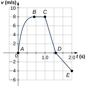
A cart is constrained to move along a straight line. A varying net force along the direction of motion is exerted on the cart. The cart's velocity v as a function of time t is shown in the graph. The five labeled points divide the graph into four sections.

Which of the following correctly ranks the magnitude of the average acceleration of the cart during the four sections of the graph?

a_CD > a_AB > a_BC > a_DE
a_BC > a_AB > a_CD > a_DE
a_AB > a_BC > a_DE > a_CD
a_CD > a_AB > a_DE > a_BC

Push a book across a table and observe it slow to a stop.

Draw graphs showing the book's position vs. time and velocity vs. time if the direction of its motion is considered positive.

Draw graphs showing the book's position vs. time and velocity vs. time if the direction of its motion is considered negative.

The position vs. time graph should be represented with a positively sloped line whose slope steadily decreases to zero. The y-intercept of the graph may be any value. The line on the velocity vs. time graph should have a positive y-intercept and a negative slope. Because the final velocity of the book is zero, the line should finish on the x-axis.

The position vs. time graph should be represented with a negatively sloped line whose slope steadily decreases to zero. The y-intercept of the graph may be any value. The line on the velocity vs. time graph should have a negative y-intercept and a positive slope. Because the final velocity of the book is zero, the line should finish on the x-axis.]

Section Summary

Acceleration is the rate at which velocity changes. In symbols, average acceleration $\bar{a}$ is
$\bar{a} = \frac{Δ v}{Δ t} = \frac{v_{f} - v_{0}}{t_{f} - t_{0}} .$
The SI unit for acceleration is $m/s squared$ .
Acceleration is a vector, and thus has a both a magnitude and direction.
Acceleration can be caused by either a change in the magnitude or the direction of the velocity.
Instantaneous acceleration $a$ is the acceleration at a specific instant in time.
Deceleration is an acceleration with a direction opposite to that of the velocity.

Conceptual Questions

Is it possible for speed to be constant while acceleration is not zero? Give an example of such a situation.

Is it possible for velocity to be constant while acceleration is not zero? Explain.

Give an example in which velocity is zero yet acceleration is not.

If a subway train is moving to the left (has a negative velocity) and then comes to a stop, what is the direction of its acceleration? Is the acceleration positive or negative?

Plus and minus signs are used in one-dimensional motion to indicate direction. What is the sign of an acceleration that reduces the magnitude of a negative velocity? Of a positive velocity?

Problems & Exercises

A cheetah can accelerate from rest to a speed of 30.0 m/s in 7.00 s. What is its acceleration?

$4. 29 m/s squared$

Professional Application

Dr. John Paul Stapp was U.S. Air Force officer who studied the effects of extreme deceleration on the human body. On December 10, 1954, Stapp rode a rocket sled, accelerating from rest to a top speed of 282 m/s (1015 km/h) in 5.00 s, and was brought jarringly back to rest in only 1.40 s! Calculate his (a) acceleration and (b) deceleration. Express each in multiples of $g$ $open parenthesis 9. 80 m /s squared close parenthesis$ by taking its ratio to the acceleration of gravity.

A commuter backs her car out of her garage with an acceleration of $1. 40 m/s squared$ . (a) How long does it take her to reach a speed of 2.00 m/s? (b) If she then brakes to a stop in 0.800 s, what is her deceleration?

(a) $1. 43 s$

(b) $minus 2. 50 m/s squared$

Assume that an intercontinental ballistic missile goes from rest to a suborbital speed of 6.50 km/s in 60.0 s (the actual speed and time are classified). What is its average acceleration in $m/s squared$ and in multiples of $g$ $open parenthesis 9. 80 m /s squared close parenthesis ?$

Adapted from College Physics 2e by OpenStax (openstax.org), licensed under CC BY-NC-SA 4.0. Changes were made. License: CC-BY-NC-SA-4.0.