9.1 Markov Chains

Chapter Overview

In this chapter, you will learn to:

Write transition matrices for Markov Chain problems.
Find the long term trend for a Regular Markov Chain.
Solve and interpret Absorbing Markov Chains.

Markov Chains

We will now study stochastic processes, experiments in which the outcomes of events depend on the previous outcomes. Such a process or experiment is called a Markov Chain or Markov process. The process was first studied by a Russian mathematician named Andrei A. Markov in the early 1900s.

A small town is served by two telephone companies, Mama Bell and Papa Bell. Due to their aggressive sales tactics, each month 40% of Mama Bell customers switch to Papa Bell, that is, the other 60% stay with Mama Bell. On the other hand, 30% of the Papa Bell customers switch to Mama Bell. The above information can be expressed in a matrix which lists the probabilities of going from one state into another state. This matrix is called a transition matrix.

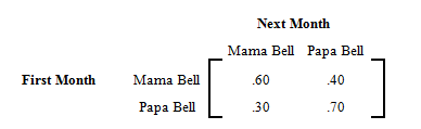
This matrix depict the flow of customers from mama bell to papa bell and vice versa. — **Figure 9.1**

The reader should observe that a transition matrix is always a square matrix because all possible states must have both rows and columns. All entries in a transition matrix are non-negative as they represent probabilities. Furthermore, since all possible outcomes are considered in the Markov process, the sum of the row entries is always 1.

Example 2

In Example 1, if it is assumed that the first day is Monday, write a matrix that gives probabilities of a transition from Monday to Wednesday.

Let $W$ denote that Professor Symons walks and $B$ denote that he rides his bicycle.

We use the following tree diagram to compute the probabilities.

Figure 9.3

The probability that Professor Symons walked on Wednesday given that he walked on Monday can be found from the tree diagram, as listed below.

$P (Walked Wednesday ∣ Walked Monday) = P (WWW) + P (WBW) = 1 / 4 + 1 / 8 = 3 / 8$ .

$P (Bicycled Wednesday ∣ Walked Monday) = P (WWB) + P (WBB) = 1 / 4 + 3 / 8 = 5 / 8$ .

$P (Walked Wednesday ∣ Bicycled Monday) = P (BWW) + P (BBW) = 1 / 8 + 3 / 16 = 3 / 5 / 16$ .

$P (Bicycled Wednesday ∣ Bicycleed Monday) = P (BWB) + P (BBB) = 1 / 8 + 9 / 16 = 11 / 16$ .

We represent the results in the following matrix.

Figure 9.4

Alternately, this result can be obtained by squaring the original transition matrix.

We list both the original transition matrix $T$ and $T^{2}$ as follows:

$T equals open bracket 1 / 2, 1 / 2; 1 / 4, 3 / 4 close bracket$

$\begin{matrix} T^{2} & [\begin{matrix} 1 / 2 & 1 / 2 \\ 1 / 4 & 3 / 4 \end{matrix}] [\begin{matrix} 1 / 2 & 1 / 2 \\ 1 / 4 & 3 / 4 \end{matrix}] \\ [\begin{matrix} 1 / 4 + 1 / 8 & 1 / 4 + 3 / 8 \\ 1 / 8 + 3 / 16 & 1 / 8 + 9 / 16 \end{matrix}] \\ [\begin{matrix} 3 / 8 & 5 / 8 \\ 5 / 16 & 11 / 16 \end{matrix}] \end{matrix}$

The reader should compare this result with the probabilities obtained from the tree diagram.

Consider the following case, for example,

$P (Walked Wednesday ∣ Bicycled Monday) = P (BWW) + P (BBW) = 1 / 8 + 3 / 16 = 5 / 16 .$

It makes sense because to find the probability that Professor Symons will walk on Wednesday given that he bicycled on Monday, we sum the probabilities of all paths that begin with $B$ and end in $W$ . There are two such paths, and they are $BWW$ and $BBW$ .

Example 3

The transition matrix for Example 1 is given below.

Figure 9.5

Write the transition matrix from a) Monday to Thursday, b) Monday to Friday.

In writing a transition matrix from Monday to Thursday, we are moving from one state to another in three steps. That is, we need to compute $T^{3}$ .

$T cubed equals open bracket 11 / 32, 21 / 32; 21 / 64, 43 / 64 close bracket$

b) To find the transition matrix from Monday to Friday, we are moving from one state to another in 4 steps. Therefore, we compute $T to the power 4$ .

$T^{4} = [\begin{matrix} 43 / 128 & 85 / 128 \\ 85 / 256 & 171 / 256 \end{matrix}]$

It is important that the student is able to interpret the above matrix correctly. For example, the entry $85 / 128$ , states that if Professor Symons walked to school on Monday, then there is $85 / 128$ probability that he will bicycle to school on Friday.

There are certain Markov chains that tend to stabilize in the long run, and they are the subject of. It so happens that the transition matrix we have used in all the above examples is just such a Markov chain. The next example deals with the long term trend or steady-state situation for that matrix.

Example 4

Suppose Professor Symons continues to walk and bicycle according to the transition matrix given in Example 1. In the long run, how often will he walk to school, and how often will he bicycle?

As mentioned earlier, as we take higher and higher powers of our matrix $T$ , it should stabilize.

$T^{5} = [\begin{matrix} . 333984 & . 666015 \\ . 333007 & . 666992 \end{matrix}]$

$T^{10} = [\begin{matrix} . 33333397 & . 66666603 \\ . 33333301 & . 66666698 \end{matrix}]$

$T^{20} = [\begin{matrix} 1 / 3 & 2 / 3 \\ 1 / 3 & 2 / 3 \end{matrix}]$

Therefore, in the long run, Professor Symons will walk to school $1 / 3$ of the time and bicycle $2 / 3$ of the time.

When this happens, we say that the system is in steady-state or state of equilibrium. In this situation, all row vectors are equal. If the original matrix is an $n$ by $n$ matrix, we get n vectors that are all the same. We call this vector a fixed probability vector or the equilibrium vector $E$ . In the above problem, the fixed probability vector $E$ is $open bracket 1 / 3, 2 / 3 close bracket$ . Furthermore, if the equilibrium vector $E$ is multiplied by the original matrix $T$ , the result is the equilibrium vector $E$ . That is,

$ET = E$

or,

$open bracket 1 / 3, 2 / 3 close bracket open bracket 1 / 2, 1 / 2; 1 / 4, 3 / 4 close bracket equals open bracket 1 / 3, 2 / 3 close bracket$

Regular Markov Chains

At the end of, we took the transition matrix $T$ and started taking higher and higher powers of it. The matrix started to stabilize, and finally it reached its steady-state or state of equilibrium. When that happened, all the row vectors became the same, and we called one such row vector a fixed probability vector or an equilibrium vector $E$ . Furthermore, we discovered that $ET = E$ .

Section Overview

In this section, we wish to answer the following four questions.

Does every Markov chain reach a state of equilibrium?
Does the product of an equilibrium vector and its transition matrix always equal the equilibrium vector? That is, does $ET = E$ ?
Can the equilibrium vector $E$ be found without raising the matrix to higher powers?
Does the long term market share distribution for a Markov chain depend on the initial market share?

Example 6

Determine whether the following Markov chains are regular.

$A equals open bracket 1, 0; .3, .7 close bracket$
$B equals open bracket 0, 1; .4, .6 close bracket$

The matrix $A$ is not a regular Markov chain because every power of it has an entry 0 in the first row, second column position. In fact, we will show that all 2 by 2 matrices that have a zero in the first row, second column position are not regular. Consider the following matrix $M$ .
$M equals open bracket a, 0; b, c close bracket$
$M^{2} = [\begin{matrix} a & 0 \\ b & c \end{matrix}] [\begin{matrix} a & 0 \\ b & c \end{matrix}] = [\begin{matrix} a \cdot a + 0 \cdot b & a \cdot 0 + 0 \cdot c \\ b \cdot a + c \cdot b & b \cdot 0 + c \cdot c \end{matrix}]$
Observe that the first row, second column entry, $a \cdot 0 + 0 \cdot c$ , will always be zero, regardless of what power we raise the matrix to.
The transition matrix $B$ is a regular Markov chain because
$B squared equals open bracket .40, .60; .24, .76 close bracket$
has only positive entries.

Example 7

Does the product of an equilibrium vector and its transition matrix always equal the equilibrium vector? That is, does $ET = E$ ?

At this point, the reader may have already guessed that the answer is yes if the transition matrix is a regular Markov chain. We try to illustrate with the following example from.

Figure 9.6

If the initial market share for Mama Bell is 20% and for Papa Bell 80%, we'd like to know the long term market share for each company.

Let matrix $T$ denote the transition matrix for this Markov chain, and $M$ denote the matrix that represents the initial market share. Then $T$ and $M$ are as follows:

$T equals open bracket .60, .40; .30, .70 close bracket$ and $M equals open bracket .20, .80 close bracket$

Since each month the towns people switch according to the transition matrix $T$ , after one month the distribution for each company is as follows:

$open bracket .20, .80 close bracket open bracket .60, .40; .30, .70 close bracket equals open bracket .36, .64 close bracket$

After two months, the market share for each company is

$open bracket .36, .64 close bracket open bracket .60, .40; .30, .70 close bracket equals open bracket .408, .592 close bracket$

After three months the distribution is

$open bracket .408, .592 close bracket open bracket .60, .40; .30, .70 close bracket equals open bracket .4224, .5776 close bracket$

After four months the market share is

$open bracket .4224, .5776 close bracket open bracket .60, .40; .30, .70 close bracket equals open bracket .42672, .57328 close bracket$

After 30 months the market share is $open bracket 3 / 7, 4 / 7 close bracket$ .

The market share after 30 months has stabilized to $open bracket 3 / 7, 4 / 7 close bracket$ .

This means that

$open bracket 3 / 7, 4 / 7 close bracket open bracket .60, .40; .30, .70 close bracket equals open bracket 3 / 7, 4 / 7 close bracket$

Once the market share reaches an equilibrium state, it stays the same, that is, $ET = E$ .

This helps us answer the next question.

Example 8

Can the equilibrium vector $E$ be found without raising the transition matrix to large powers?

The answer to the second question provides us with a way to find the equilibrium vector $E$ .

The answer lies in the fact that $ET = E$ .

Since we have the matrix $T$ , we can determine $E$ from the statement $ET = E$ .

Suppose $E = [\begin{matrix} e & 1 - e \end{matrix}]$ , then $ET = E$ gives us

$[\begin{matrix} e & 1 - e \end{matrix}] [\begin{matrix} . 60 & . 40 \\ . 30 & . 70 \end{matrix}] = [\begin{matrix} e & 1 - e \end{matrix}]$

$[\begin{matrix} (. 60) e + . 30 (1 - e) & (. 40) e + . 70 (1 - e) \end{matrix}] = [\begin{matrix} e & 1 - e \end{matrix}]$

$[\begin{matrix} . 30 e + . 30 & - . 30 e + . 70 \end{matrix}] = [\begin{matrix} e & 1 - e \end{matrix}]$

$. 30 e + . 30 = e$

$e equals 3 / 7$

Therefore, $E equals open bracket 3 / 7, 4 / 7 close bracket$

Example 9

Does the long term market share for a Markov chain depend on the initial market share?

We will show that the final market share distribution for a Markov chain does not depend upon the initial market share. In fact, one does not even need to know the initial market share distribution to find the long term distribution. Furthermore, the final market share distribution can be found by simply raising the transition matrix to higher powers.

Consider the initial market share $open bracket .20, .80 close bracket$ , and the transition matrix $T equals open bracket .60, .40; .30, .70 close bracket$ for Mama Bell and Papa Bell in the above example. Recall we found $T^{n}$ , for very large $n$ , to be $open bracket 3 / 7, 4 / 7; 3 / 7, 4 / 7 close bracket$ .

Clearly, $open bracket .20, .80 close bracket open bracket 3 / 7, 4 / 7; 3 / 7, 4 / 7 close bracket equals open bracket 3 / 7, 4 / 7 close bracket$

No matter what the initial market share, the product is $open bracket 3 / 7, 4 / 7 close bracket$ .

If the initial share is $open bracket .10, .90 close bracket$ , then

$open bracket .10, .90 close bracket open bracket 3 / 7, 4 / 7; 3 / 7, 4 / 7 close bracket equals open bracket 3 / 7, 4 / 7 close bracket$

For any distribution $A = [\begin{matrix} a & 1 - a \end{matrix}]$ , for example,

$[\begin{matrix} a & 1 - a \end{matrix}] [\begin{matrix} 3 / 7 & 4 / 7 \\ 3 / 7 & 4 / 7 \end{matrix}] = [\begin{matrix} 3 / 7 (a) + 3 / 7 (1 - a) & 4 / 7 (a) + 4 / 7 (1 - a) \end{matrix}] = [\begin{matrix} 3 / 7 & 4 / 7 \end{matrix}]$

It makes sense, because the entry $3 / 7 (a) + 3 / 7 (1 - a)$ , for example, will always equal $3 / 7$ .

Just as the sum of the parts equals the whole, the sum of the parts of $3 / 7$ equals $3 / 7$ .

We summarize as follows:

Regular Markov Chains A Markov chain is said to be a Regular Markov chain if some power of it has only positive entries.
Let $T$ be a transition matrix for a regular Markov chain.

As we take higher powers of $T$ , $T^{n}$ , as n becomes large, approaches a state of equilibrium.
If $M$ is any distribution vector, and $E$ an equilibrium vector, then ${MT}^{n} = E$ .
Each row of the equilibrium matrix $T^{n}$ is a unique equilibrium vector $E$ such that $ET = E$ .
The equilibrium distribution vector $E$ can be found by letting $ET = E$ .

Absorbing Markov Chains

In this section, we will study a type of Markov chain in which when a certain state is reached, it is impossible to leave that state. Such states are called absorbing states, and a Markov Chain that has at least one such state is called an Absorbing Markov chain. Suppose you have the following transition matrix.

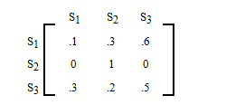
This matrix depicts the probability of moving from one sate to the other. — **Figure 9.8**

The state $S sub 2$ is an absorbing state, because the probability of moving from state $S sub 2$ to state $S sub 2$ is 1. Which is another way of saying that if you are in state $S sub 2$ , you will remain in state $S sub 2$ .

In fact, this is the way to identify an absorbing state. If the probability in row i and column i, $p_{ii}$ , is 1, then state $S_{i}$ is an absorbing state.

We begin with an application of absorbing Markov chains to the gambler's ruin problem.

Example 11 Gambler's Ruin Problem

A gambler has $3,000, and she decides to gamble $1,000 at a time at a Black Jack table in a casino in Las Vegas. She has told herself that she will continue playing until she goes broke or has $5,000. Her probability of winning at Black Jack is $.40$ . Write the transition matrix, identify the absorbing states, find the solution matrix, and determine the probability that the gambler will be financially ruined at a stage when she has $2,000.

The transition matrix is written below. Clearly the state 0 and state $5K$ are the absorbing states. This makes sense because as soon as the gambler reaches 0, she is financially ruined and the game is over. Similarly, if the gambler reaches $5,000, she has promised herself to quit and, again, the game is over. The reader should note that $p sub 00 equals 1$ , and $p sub 55 equals 1$ .

Further observe that since the gambler bets only $1,000 at a time, she can raise or lower her money only by $1,000 at a time. In other words, if she has $2,000 now, after the next bet she can have $3,000 with a probability of $.40$ and $1,000 with a probability of $.60$ .

Figure 9.9

To determine the long term trend, we raise the matrix to higher powers until all the non- absorbing states are absorbed. This is the called the solution matrix.

Figure 9.10

The solution matrix is often written in the following form, where the non-absorbing states are written as rows on the side, and the absorbing states as columns on the top.

Figure 9.11

The table lists the probabilities of getting absorbed in state 0 or state 5K starting from any of the four non-absorbing states. For example, if at any instance the gambler has $3,000, then her probability of financial ruin is 135/211.

Example 12

Solve the Gambler's Ruin Problem of Example 11 without raising the matrix to higher powers, and determine the number of bets the gambler makes before the game is over.

In solving absorbing states, it is often convenient to rearrange the matrix so that the rows and columns corresponding to the absorbing states are listed first. This is called the Canonical form. The transition matrix of Example 11 in the canonical form is listed below.

Figure 9.12

The canonical form divides the transition matrix into four sub-matrices as listed below.

Figure 9.13

The matrix $F = {(1_{n} - B)}^{- 1}$ is called the fundamental matrix for the absorbing Markov chain, where $I_{n}$ is an identity matrix of the same size as $B$ . The $i$ , $j - th$ entry of this matrix tells us the average number of times the process is in the non-absorbing state $j$ before absorption if it started in the non-absorbing state $i$ . The matrix $F$ for our problem is listed below.

Figure 9.14

The Fundamental matrix $F$ helps us determine the average number of games played before absorption.

According to the matrix, the entry 1.78 in the row 3, column 2 position says that the gambler will play the game 1.78 times before she goes from $3K to $2K. The entry 2.25 in row 3, column 3 says that if the gambler now has $3K, she will have $3K on the average 2.25 times before the game is over.

We now address the question of how many bets will she have to make before she is absorbed, if the gambler begins with $3K?

If we add the number of games the gambler plays in each non-absorbing state, we get the average number of games before absorption from that state. Therefore, if the gambler starts with $3K, the average number of Black Jack games she will play before absorption is

$1 . 07 + 1 . 78 + 2 . 25 + . 90 = 6 . 0$

That is, we expect the gambler will either have $5,000 or nothing on the 7th bet.

Lastly, we find the solution matrix without raising the transition matrix to higher powers.

The matrix $FA$ gives us the solution matrix.

$FA = [\begin{matrix} 1.54 & . 90 & . 47 & . 19 \\ 1.35 & 2.25 & 1.18 & . 47 \\ 1.07 & 1.78 & 2.25 & . 90 \\ . 64 & 1.07 & 1.35 & 1.54 \end{matrix}] [\begin{matrix} . 6 & 0 \\ 0 & 0 \\ 0 & 0 \\ 0 & . 4 \end{matrix}] = [\begin{matrix} . 92 & . 08 \\ . 81 & . 19 \\ . 64 & . 36 \\ . 38 & . 62 \end{matrix}]$

Which is the same as the following matrix we obtained by raising the transition matrix to higher powers.

Figure 9.15

We summarize as follows:

Absorbing Markov Chains

A Markov chain is an absorbing Markov chain if it has at least one absorbing state. A state $i$ is an absorbing state if once the system reaches state $i$ , it stays in that state; that is, $p sub ii equals 1$ .
If a transition matrix $T$ for an absorbing Markov chain is raised to higher powers, it reaches an absorbing state called the solution matrix and stays there. The $i$ , $j - th$ entry of this matrix gives the probability of absorption in state $j$ while starting in state $i$ .
Alternately, the solution matrix can be found in the following manner.
1. Express the transition matrix in the canonical form as below.
  $T equals open bracket I sub n, 0; A, B close bracket$
  
  where $I_{n}$ is an identity matrix, and 0 is a matrix of all zeros.
2. The fundamental matrix $F = {(I - B)}^{- 1}$ . The fundamental matrix helps us find the number of games played before absorption.
3. $FA$ is the solution matrix, whose $i$ , $j - th$ entry gives the probability of absorption in state $j$ while starting in state $i$ .
The sum of the entries of a row of the fundamental matrix gives us the expected number of steps before absorption for the non-absorbing state associated with that row.

Adapted from Applied Finite Mathematics by Rupinder Sekhon (De Anza College), originally published by OpenStax CNX (cnx.org, collection col10613), licensed under CC BY 3.0. Changes were made. License: CC-BY-3.0.