8.3 Calculating the RM ANOVA

Now that you are familiar with the concept of an ANOVA table (remember the table from last chapter where we reported all of the parts to calculate the $F$-value?), we can take a look at the things we need to find out to make the ANOVA table. Figure 8.3 presents an abstract for the repeated-measures ANOVA table. It shows us all the thing we need to calculate to get the $F$-value for our data.

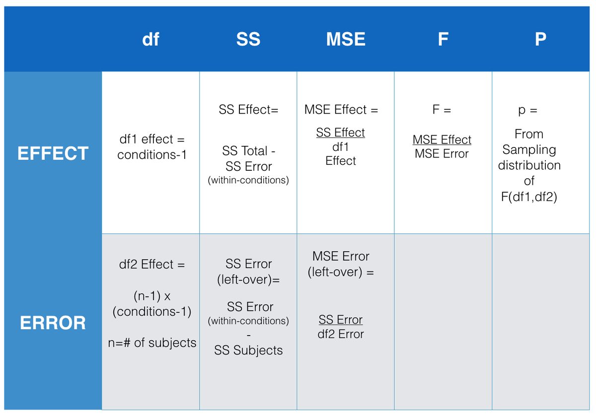
So, what we need to do is calculate all the $SS$es that we did before for the between-subjects ANOVA. That means the next three steps are identical to the ones you did before. In fact, I will just basically copy the next three steps to find $S{S}_{\text{TOTAL}}$, $S{S}_{\text{Effect}}$, and $S{S}_{\text{Error (within-conditions)}}$. After that we will talk about splitting up $S{S}_{\text{Error (within-conditions)}}$ into two parts, this is the new thing for this chapter. Here we go!

8.3.1 SS Total

The total sums of squares, or $SS\text{Total}$ measures the total variation in a set of data. All we do is find the difference between each score and the grand mean, then we square the differences and add them all up.

The mean of all of the scores is called the Grand Mean. It’s calculated in the table, the Grand Mean = 7.

We also calculated all of the difference scores from the Grand Mean. The difference scores are in the column titled diff. Next, we squared the difference scores, and those are in the next column called diff_squared.

When you add up all of the individual squared deviations (difference scores) you get the sums of squares. That’s why it’s called the sums of squares (SS).

Now, we have the first part of our answer:

$$S{S}_{\text{total}}=S{S}_{\text{Effect}}+S{S}_{\text{Error}}$$

$S{S}_{\text{total}}=302$ and

$$302=S{S}_{\text{Effect}}+S{S}_{\text{Error}}$$

8.3.2 SS Effect

$S{S}_{\text{Total}}$ gave us a number representing all of the change in our data, how they all are different from the grand mean.

What we want to do next is estimate how much of the total change in the data might be due to the experimental manipulation. For example, if we ran an experiment that causes causes change in the measurement, then the means for each group will be different from other, and the scores in each group will be different from each. As a result, the manipulation forces change onto the numbers, and this will naturally mean that some part of the total variation in the numbers is caused by the manipulation.

The way to isolate the variation due to the manipulation (also called effect) is to look at the means in each group, and the calculate the difference scores between each group mean and the grand mean, and then the squared deviations to find the sum for $S{S}_{\text{Effect}}$.

Consider this table, showing the calculations for $S{S}_{\text{Effect}}$.

Notice we created a new column called means, these are the means for each condition, A, B, and C.

$S{S}_{\text{Effect}}$ represents the amount of variation that is caused by differences between the means. The diff column is the difference between each condition mean and the grand mean, so for the first row, we have 11-7 = 4, and so on.

We found that $S{S}_{\text{Effect}}=72$, this is the same as the ANOVA from the previous chapter

8.3.3 SS Error (within-conditions)

Great, we made it to SS Error. We already found SS Total, and SS Effect, so now we can solve for SS Error just like this:

$$S{S}_{\text{total}}=S{S}_{\text{Effect}}+S{S}_{\text{Error (within-conditions)}}$$

switching around:

$ SS_ = SS_ - SS_ $

$ SS_ = 302 - 72 = 230 $

Or, we could compute $S{S}_{\text{Error (within conditions)}}$ directly from the data as we did last time:

When we compute $S{S}_{\text{Error (within conditions)}}$ directly, we find the difference between each score and the condition mean for that score. This gives us the remaining error variation around the condition mean, that the condition mean does not explain.

8.3.4 SS Subjects

Now we are ready to calculate new partition, called $S{S}_{\text{Subjects}}$. We first find the means for each subject. For subject 1, this is the mean of their scores across Conditions A, B, and C. The mean for subject 1 is 9.33 (repeating). Notice there is going to be some rounding error here, that’s OK for now.

The means column now shows all of the subject means. We then find the difference between each subject mean and the grand mean. These deviations are shown in the diff column. Then we square the deviations, and sum them up.

We found that the sum of the squared deviations $S{S}_{\text{Subjects}}$ = 52.75. Note again, this has some small rounding error because some of the subject means had repeating decimal places, and did not divide evenly.

We can see the effect of the rounding error if we look at the sum and mean in the diff column. We know these should be both zero, because the Grand mean is the balancing point in the data. The sum and mean are both very close to zero, but they are not zero because of rounding error.

8.3.5 SS Error (left-over)

Now we can do the last thing. Remember we wanted to split up the $S{S}_{\text{Error (within conditions)}}$ into two parts, $S{S}_{\text{Subjects}}$ and $S{S}_{\text{Error (left-over)}}$. Because we have already calculate $S{S}_{\text{Error (within conditions)}}$ and $S{S}_{\text{Subjects}}$, we can solve for $S{S}_{\text{Error (left-over)}}$:

$$S{S}_{\text{Error (left-over)}}=S{S}_{\text{Error (within conditions)}}-S{S}_{\text{Subjects}}$$

$$S{S}_{\text{Error (left-over)}}=S{S}_{\text{Error (within conditions)}}-S{S}_{\text{Subjects}}=230-52.75=177.25$$

8.3.6 Check our work

Before we continue to compute the MSEs and F-value for our data, let’s quickly check our work. For example, we could have R compute the repeated measures ANOVA for us, and then we could look at the ANOVA table and see if we are on the right track so far.

Table 8.3 looks good. We found the $S{S}_{\text{Effect}}$ to be 72, and the SS for the conditions (same thing) in the table is also 72. We found the $S{S}_{\text{Subjects}}$ to be 52.75, and the SS for the first residual (same thing) in the table is also 53.66 repeating. That’s close, and our number is off because of rounding error. Finally, we found the $S{S}_{\text{Error (left-over)}}$ to be 177.25, and the SS for the bottom residuals in the table (same thing) in the table is 177.33 repeating, again close but slightly off due to rounding error.

We have finished our job of computing the sums of squares that we need in order to do the next steps, which include computing the MSEs for the effect and the error term. Once we do that, we can find the F-value, which is the ratio of the two MSEs.

Before we do that, you may have noticed that we solved for $S{S}_{\text{Error (left-over)}}$, rather than directly computing it from the data. In this chapter we are not going to show you the steps for doing this. We are not trying to hide anything from, instead it turns out these steps are related to another important idea in ANOVA. We discuss this idea, which is called an interaction in the next chapter, when we discuss factorial designs (designs with more than one independent variable).

8.3.7 Compute the MSEs

Calculating the MSEs (mean squared error) that we need for the $F$-value involves the same general steps as last time. We divide each SS by the degrees of freedom for the SS.

The degrees of freedom for $S{S}_{\text{Effect}}$ are the same as before, the number of conditions - 1. We have three conditions, so the df is 2. Now we can compute the $MS{E}_{\text{Effect}}$.

$$MS{E}_{\text{Effect}}=\frac{S{S}_{\text{Effect}}}{df}=\frac{72}{2}=36$$

The degrees of freedom for $S{S}_{\text{Error (left-over)}}$ are different than before, they are the (number of subjects - 1) multiplied by the (number of conditions -1). We have 3 subjects and three conditions, so $(3-1)*(3-1)=2*2=4$. You might be wondering why we are multiplying these numbers. Hold that thought for now and wait until the next chapter. Regardless, now we can compute the $MS{E}_{\text{Error (left-over)}}$.

$$MS{E}_{\text{Error (left-over)}}=\frac{S{S}_{\text{Error (left-over)}}}{df}=\frac{177.33}{4}=44.33$$

8.3.8 Compute F

We just found the two MSEs that we need to compute $F$. We went through all of this to compute $F$ for our data, so let’s do it:

$$F=\frac{MS{E}_{\text{Effect}}}{MS{E}_{\text{Error (left-over)}}}=\frac{36}{44.33}=0.812$$

And, there we have it!

8.3.9 p-value

We already conducted the repeated-measures ANOVA using R and reported the ANOVA. Here it is again. The table shows the $p$-value associated with our $F$-value.

We might write up the results of our experiment and say that the main effect condition was not significant, F(2,4) = 0.812, MSE = 44.33, p = 0.505.

What does this statement mean? Remember, that the $p$-value represents the probability of getting the $F$ value we observed or larger under the null (assuming that the samples come from the same distribution, the assumption of no differences). So, we know that an $F$-value of 0.812 or larger happens fairly often by chance (when there are no real differences), in fact it happens 50.5% of the time. As a result, we do not reject the idea that any differences in the means we have observed could have been produced by chance.

Adapted from Answering Questions with Data: Introductory Statistics for Psychology Students, by Matthew J. C. Crump (Brooklyn College of CUNY), crumplab.com/statistics, licensed under CC BY-SA 4.0. Portions adapt Danielle Navarro's Learning Statistics with R (CC BY-SA). Changes were made; this adaptation is distributed under the same license. License: CC-BY-SA-4.0.