8.2 Partitioning the Sums of Squares

Time to introduce a new name for an idea you learned about last chapter, it’s called partitioning the sums of squares. Sometimes an obscure new name can be helpful for your understanding of what is going on. ANOVAs are all about partitioning the sums of squares. We already did some partitioning in the last chapter. What do we mean by partitioning?

Imagine you had a big empty house with no rooms in it. What would happen if you partitioned the house? What would you be doing? One way to partition the house is to split it up into different rooms. You can do this by adding new walls and making little rooms everywhere. That’s what partitioning means, to split up.

The act of partitioning, or splitting up, is the core idea of ANOVA. To use the house analogy. Our total sums of squares (SS Total) is our big empty house. We want to split it up into little rooms. Before we partitioned SS Total using this formula:

$$S{S}_{\text{TOTAL}}=S{S}_{\text{Effect}}+S{S}_{\text{Error}}$$

Remember, the $S{S}_{\text{Effect}}$ was the variance we could attribute to the means of the different groups, and $S{S}_{\text{Error}}$ was the leftover variance that we couldn’t explain. $S{S}_{\text{Effect}}$ and $S{S}_{\text{Error}}$ are the partitions of $S{S}_{\text{TOTAL}}$, they are the little rooms.

In the between-subjects case above, we got to split $S{S}_{\text{TOTAL}}$ into two parts. What is most interesting about the repeated-measures design, is that we get to split $S{S}_{\text{TOTAL}}$ into three parts, there’s one more partition. Can you guess what the new partition is? Hint: whenever we have a new way to calculate means in our design, we can always create a partition for those new means. What are the new means in the repeated measures design?

Here is the new idea for partitioning $S{S}_{\text{TOTAL}}$ in a repeated-measures design:

$$S{S}_{\text{TOTAL}}=S{S}_{\text{Effect}}+S{S}_{\text{Subjects}}+S{S}_{\text{Error}}$$

We’ve added $S{S}_{\text{Subjects}}$ as the new idea in the formula. What’s the idea here? Well, because each subject was measured in each condition, we have a new set of means. These are the means for each subject, collapsed across the conditions. For example, subject 1 has a mean (mean of their scores in conditions A, B, and C); subject 2 has a mean (mean of their scores in conditions A, B, and C); and subject 3 has a mean (mean of their scores in conditions A, B, and C). There are three subject means, one for each subject, collapsed across the conditions. And, we can now estimate the portion of the total variance that is explained by these subject means.

We just showed you a “formula” to split up $S{S}_{\text{TOTAL}}$ into three parts, but we called the formula an idea. We did that because the way we wrote the formula is a little bit misleading, and we need to clear something up. Before we clear the thing up, we will confuse you just a little bit. Be prepared to be confused a little bit.

First, we need to introduce you to some more terms. It turns out that different authors use different words to describe parts of the ANOVA. This can be really confusing. For example, we described the SS formula for a between subjects design like this:

$$S{S}_{\text{TOTAL}}=S{S}_{\text{Effect}}+S{S}_{\text{Error}}$$

However, the very same formula is often written differently, using the words between and within in place of effect and error, it looks like this:

$$S{S}_{\text{TOTAL}}=S{S}_{\text{Between}}+S{S}_{\text{Within}}$$

Whoa, hold on a minute. Haven’t we switched back to talking about a between-subjects ANOVA. YES! Then why are we using the word within, what does that mean? YES! We think this is very confusing for people. Here the word within has a special meaning. It does not refer to a within-subjects design. Let’s explain. First, $S{S}_{\text{Between}}$ (which we have been calling $S{S}_{\text{Effect}}$) refers to variation between the group means, that’s why it is called $S{S}_{\text{Between}}$. Second, and most important, $S{S}_{\text{Within}}$ (which we have been calling $S{S}_{\text{Error}}$), refers to the leftover variation within each group mean. Specifically, it is the variation between each group mean and each score in the group. “AAGGH, you’ve just used the word between to describe within group variation!”. Yes! We feel your pain. Remember, for each group mean, every score is probably off a little bit from the mean. So, the scores within each group have some variation. This is the within group variation, and it is why the leftover error that we can’t explain is often called $S{S}_{\text{Within}}$.

OK. So why did we introduce this new confusing way of talking about things? Why can’t we just use $S{S}_{\text{Error}}$ to talk about this instead of $S{S}_{\text{Within}}$, which you might (we do) find confusing. We’re getting there, but perhaps Figure 8.1 will help out.

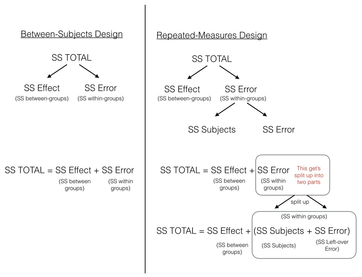
The figure lines up the partitioning of the Sums of Squares for both between-subjects and repeated-measures designs. In both designs, $S{S}_{\text{Total}}$ is first split up into two pieces $S{S}_{\text{Effect (between-groups)}}$ and $S{S}_{\text{Error (within-groups)}}$. At this point, both ANOVAs are the same. In the repeated measures case we split the $S{S}_{\text{Error (within-groups)}}$ into two more littler parts, which we call $$S{S}_{\text{Subjects (error variation about the subject mean)}}$$ and $$S{S}_{\text{Error (left-over variation we can't explain)}}$$.

So, when we earlier wrote the formula to split up SS in the repeated-measures design, we were kind of careless in defining what we actually meant by $S{S}_{\text{Error}}$, this was a little too vague:

$$S{S}_{\text{TOTAL}}=S{S}_{\text{Effect}}+S{S}_{\text{Subjects}}+S{S}_{\text{Error}}$$

The critical feature of the repeated-measures ANOVA, is that the $S{S}_{\text{Error}}$ that we will later use to compute the MSE in the denominator for the $F$-value, is smaller in a repeated-measures design, compared to a between subjects design. This is because the $S{S}_{\text{Error (within-groups)}}$ is split into two parts, $$S{S}_{\text{Subjects (error variation about the subject mean)}}$$ and $$S{S}_{\text{Error (left-over variation we can't explain)}}$$.

To make this more clear, consider Figure 8.2:

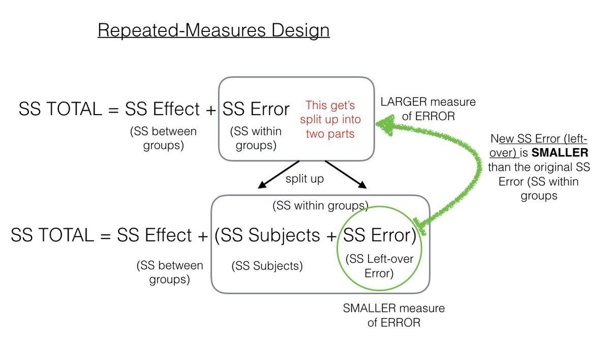
As we point out, the $S{S}_{\text{Error (left-over)}}$ in the green circle will be a smaller number than the $S{S}_{\text{Error (within-group)}}$. That’s because we are able to subtract out the $S{S}_{\text{Subjects}}$ part of the $S{S}_{\text{Error (within-group)}}$. As we will see shortly, this can have the effect of producing larger F-values when using a repeated-measures design compared to a between-subjects design.

Adapted from Answering Questions with Data: Introductory Statistics for Psychology Students, by Matthew J. C. Crump (Brooklyn College of CUNY), crumplab.com/statistics, licensed under CC BY-SA 4.0. Portions adapt Danielle Navarro's Learning Statistics with R (CC BY-SA). Changes were made; this adaptation is distributed under the same license. License: CC-BY-SA-4.0.