7.5 The Quantum Harmonic Oscillator

The Classic Harmonic Oscillator

A simple harmonic oscillator is a particle or system that undergoes harmonic motion about an equilibrium position, such as an object with mass vibrating on a spring. In this section, we consider oscillations in one-dimension only. Suppose a mass moves back-and-forth along the

x-direction about the equilibrium position, $x=0$. In classical mechanics, the particle moves in response to a linear restoring force given by $F_x=\text{−}kx,$ where x is the displacement of the particle from its equilibrium position. The motion takes place between two turning points, $x=\text{±}A$, where A denotes the amplitude of the motion. The position of the object varies periodically in time with angular frequency $\omega =\sqrt{k\text{/}m},$ which depends on the mass m of the oscillator and on the force constant k of the net force, and can be written as

$$x(t)=A\text{cos}(\omega t+\varphi ).$$

The total energy E of an oscillator is the sum of its kinetic energy $K=m{u}^2\text{/}2$ and the elastic potential energy of the force $U(x)=k{x}^2\text{/}2,$

At turning points $x=\text{±}A$, the speed of the oscillator is zero; therefore, at these points, the energy of oscillation is solely in the form of potential energy $E=k{A}^2\text{/}2$. The plot of the potential energy U(x) of the oscillator versus its position x is a parabola (Figure 7.13). The potential-energy function is a quadratic function of x, measured with respect to the equilibrium position. On the same graph, we also plot the total energy E of the oscillator, as a horizontal line that intercepts the parabola at $x=\text{±}A$. Then the kinetic energy K is represented as the vertical distance between the line of total energy and the potential energy parabola.

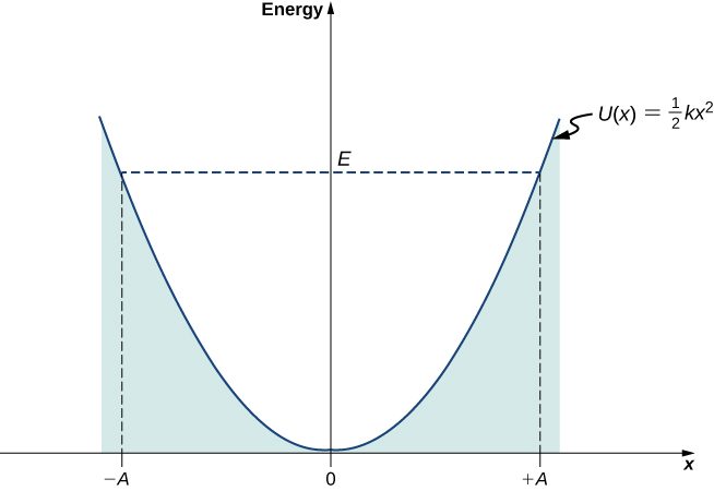
In this plot, the motion of a classical oscillator is confined to the region where its kinetic energy is nonnegative, which is what the energy relation Equation 7.53 says. Physically, it means that a classical oscillator can never be found beyond its turning points, and its energy depends only on how far the turning points are from its equilibrium position. The energy of a classical oscillator changes in a continuous way. The lowest energy that a classical oscillator may have is zero, which corresponds to a situation where an object is at rest at its equilibrium position. The zero-energy state of a classical oscillator simply means no oscillations and no motion at all (a classical particle sitting at the bottom of the potential well in Figure 7.13). When an object oscillates, no matter how big or small its energy may be, it spends the longest time near the turning points, because this is where it slows down and reverses its direction of motion. Therefore, the probability of finding a classical oscillator between the turning points is highest near the turning points and lowest at the equilibrium position. (Note that this is not a statement of preference of the object to go to lower energy. It is a statement about how quickly the object moves through various regions.)

The Quantum Harmonic Oscillator

One problem with this classical formulation is that it is not general. We cannot use it, for example, to describe vibrations of diatomic molecules, where quantum effects are important. A first step toward a quantum formulation is to use the classical expression $k=m{\omega }^2$ to limit mention of a “spring” constant between the atoms. In this way the potential energy function can be written in a more general form,

$$U(x)=\frac{1}{2}m{\omega }^2{x}^2.$$

Combining this expression with the time-independent Schrӧdinger equation gives

To solve Equation 7.55—that is, to find the allowed energies E and their corresponding wave functions $\psi (x)$ —we require the wave functions to be symmetric about $x=0$ (the bottom of the potential well) and to be normalizable. These conditions ensure that the probability density $|\psi (x){|}^2$ must be finite when integrated over the entire range of x from $\text{−}\infty$ to $+\infty$. How to solve Equation 7.55 is the subject of a more advanced course in quantum mechanics; here, we simply cite the results. The allowed energies are

The wave functions that correspond to these energies (the stationary states or states of definite energy) are

where $\beta =\sqrt{m\omega \text{/}\hslash }$, $N_n$ is the normalization constant, and $H_n(y)$ is a polynomial of degree n called a Hermite polynomial. The first four Hermite polynomials are

$$\begin{array}{c}{H}_0\left(y\right)=1\hfill \\ H_1\left(y\right)=2y\hfill \\ H_2\left(y\right)=4y^2-2\hfill \\ H_3\left(y\right)=8y^3-12y.\hfill \end{array}$$

A few sample wave functions are given in Figure 7.14. As the value of the principal number increases, the solutions alternate between even functions and odd functions about $x=0$.

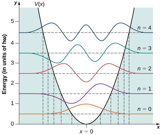
Several interesting features appear in this solution. Unlike a classical oscillator, the measured energies of a quantum oscillator can have only energy values given by Equation 7.56. Moreover, unlike the case for a quantum particle in a box, the allowable energy levels are evenly spaced,

When a particle bound to such a system makes a transition from a higher-energy state to a lower-energy state, the smallest-energy quantum carried by the emitted photon is necessarily hf. Similarly, when the particle makes a transition from a lower-energy state to a higher-energy state, the smallest-energy quantum that can be absorbed by the particle is hf. A quantum oscillator can absorb or emit energy only in multiples of this smallest-energy quantum. This is consistent with Planck’s hypothesis for the energy exchanges between radiation and the cavity walls in the blackbody radiation problem.

The quantum oscillator differs from the classic oscillator in three ways:

First, the ground state of a quantum oscillator is $E_0=\hslash \omega \text{/}2,$ not zero. In the classical view, the lowest energy is zero. The nonexistence of a zero-energy state is common for all quantum-mechanical systems because of omnipresent fluctuations that are a consequence of the Heisenberg uncertainty principle. If a quantum particle sat motionless at the bottom of the potential well, its momentum as well as its position would have to be simultaneously exact, which would violate the Heisenberg uncertainty principle. Therefore, the lowest-energy state must be characterized by uncertainties in momentum and in position, so the ground state of a quantum particle must lie above the bottom of the potential well.

Second, a particle in a quantum harmonic oscillator potential can be found with nonzero probability outside the interval $\text{−}A\le x\le +A$. In a classic formulation of the problem, the particle would not have any energy to be in this region. The probability of finding a ground-state quantum particle in the classically forbidden region is about 16%.

Third, the probability density distributions $|{\psi }_n(x){|}^2$ for a quantum oscillator in the ground low-energy state, ${\psi }_0(x)$, is largest at the middle of the well $(x=0)$. For the particle to be found with greatest probability at the center of the well, we expect that the particle spends the most time there as it oscillates. This is opposite to the behavior of a classical oscillator, in which the particle spends most of its time moving with relative small speeds near the turning points.

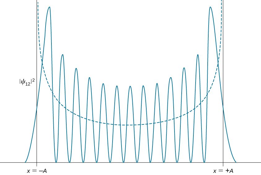
Quantum probability density distributions change in character for excited states, becoming more like the classical distribution when the quantum number gets higher. We observe this change already for the first excited state of a quantum oscillator because the distribution $|{\psi }_1(x){|}^2$ peaks up around the turning points and vanishes at the equilibrium position, as seen in Figure 7.13. In accordance with Bohr’s correspondence principle, in the limit of high quantum numbers, the quantum description of a harmonic oscillator converges to the classical description, which is illustrated in Figure 7.15. The classical probability density distribution corresponding to the quantum energy of the $n=12$ state is a reasonably good approximation of the quantum probability distribution for a quantum oscillator in this excited state. This agreement becomes increasingly better for highly excited states.

Summary

• The quantum harmonic oscillator is a model built in analogy with the model of a classical harmonic oscillator. It models the behavior of many physical systems, such as molecular vibrations or wave packets in quantum optics.
• The allowed energies of a quantum oscillator are discrete and evenly spaced. The energy spacing is equal to Planck’s energy quantum.
• The ground state energy is larger than zero. This means that, unlike a classical oscillator, a quantum oscillator is never at rest, even at the bottom of a potential well, and undergoes quantum fluctuations.
• The stationary states (states of definite energy) have nonzero values also in regions beyond classical turning points. When in the ground state, a quantum oscillator is most likely to be found around the position of the minimum of the potential well, which is the least-likely position for a classical oscillator.
• For high quantum numbers, the motion of a quantum oscillator becomes more similar to the motion of a classical oscillator, in accordance with Bohr’s correspondence principle.

Conceptual Questions

Problems