7.1 Wave Functions

In the preceding chapter, we saw that particles act in some cases like particles and in other cases like waves. But what does it mean for a particle to “act like a wave”? What precisely is “waving”? What rules govern how this wave changes and propagates? How is the wave function used to make predictions? For example, if the amplitude of an electron wave is given by a function of position and time, $Ψ (x, t)$ , defined for all x, where exactly is the electron? The purpose of this chapter is to answer these questions.

Using the Wave Function

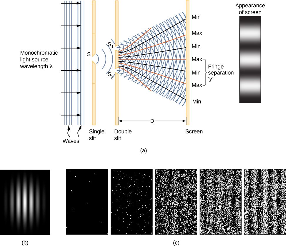
A clue to the physical meaning of the wave function $Ψ (x, t)$ is provided by the two-slit interference of monochromatic light (Figure 7.2). (See also Electromagnetic Waves and Interference.) The wave function of a light wave is given by E(x,t), and its energy density is given by $| E | squared$ , where E is the electric field strength. The energy of an individual photon depends only on the frequency of light, $ε_{photon} = h f,$ so $| E | squared$ is proportional to the number of photons. When light waves from $S sub 1$ interfere with light waves from $S sub 2$ at the viewing screen (a distance D away), an interference pattern is produced (part (a) of the figure). Bright fringes correspond to points of constructive interference of the light waves, and dark fringes correspond to points of destructive interference of the light waves (part (b)).

Suppose the screen is initially unexposed to light. If the screen is exposed to very weak light, the interference pattern appears gradually (Figure 7.2(c), left to right). Individual photon hits on the screen appear as dots. The dot density is expected to be large at locations where the interference pattern will be, ultimately, the most intense. In other words, the probability (per unit area) that a single photon will strike a particular spot on the screen is proportional to the square of the total electric field, $| E | squared$ at that point. Under the right conditions, the same interference pattern develops for matter particles, such as electrons.

Part a shows monochromatic light of wavelength lambda emitted from a source, arriving as plane waves at a single slit, S. The waves pass through the slit ad form circular waves that arrive at a double slit, S sub 1 and S sub 2. The light rays emerge from two slits as semicircles overlapping one another. The interacting waves spread out and end on a screen where points of maximum, where the crests or troughs overlap, and minimum, where the crests from one slit overlap the troughs from the other, are marked. The pattern appears on the screen as a series of alternating bright and dark fringes. The fringes separation, y, is the distance between adjacent maxima. In part b, a photograph of the fringe pattern is shown. Part c shows how the pattern develops in time. Photos of the image at five times are shown. At first, only a few scattered bright points appear, apparently randomly, against a dark background. In the second image, we see more dots but not yet any discernible pattern. In the third image, we start to see that there are more dots in some parts of the image and fewer elsewhere. Vertical stripes of dense bright dots separated are clearly seen in the fourth image, and even more clearly in the fifth. — **Figure 7.2** Two-slit interference of monochromatic light. (a) Schematic of two-slit interference; (b) light interference pattern; (c) interference pattern built up gradually under low-intensity light (left to right).

The square of the matter wave $| Ψ | squared$ in one dimension has a similar interpretation as the square of the electric field $| E | squared$ . It gives the probability that a particle will be found at a particular position and time per unit length, also called the probability density. The probability (P) a particle is found in a narrow interval (x, x + dx) at time t is therefore

$P (x, x + d x) = | Ψ (x, t) |^{2} d x .$

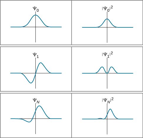
(Later, we define the magnitude squared for the general case of a function with “imaginary parts.”) This probabilistic interpretation of the wave function is called the Born interpretation. Examples of wave functions and their squares for a particular time t are given in Figure 7.3.

Three wave functions and the square of the amplitude of the wave functions. The first wave function, psi sub zero, and its square are symmetric, positive, peaked at x = 0, and zero far from the origin. The second wave function, psi sub 1, is antisymmetric: the function is negative at negative x, positive at positive x, and zero at the origin as well as plus and minus infinity. There is a negative minimum at negative x and positive maximum at positive x. The minimum value is exactly opposite the maximum value. The square of the amplitude of the wave function is positive and symmetric about the origin, where the value is zero, with a maximum on either side of the origin. The third wave function, psi sub N, is not symmetric. It is zero at minus infinity, decreases to a negative minimum value at some x less than zero, crosses zero, still at x less than zero, and becomes positive. It reaches a positive maximum at some positive x, then decreases to zero at large x. The minimum value is smaller in magnitude than the maximum value. The square of the amplitude of the wave function is positive, with two local maxima. The first maximum is smaller and at negative x, and the second is larger and at positive x. The square of the function is zero at one point between the maxima. — **Figure 7.3** Several examples of wave functions and the corresponding square of their wave functions.

If the wave function varies slowly over the interval $Δ x$ , the probability a particle is found in the interval is approximately

$P (x, x + Δ x) \approx | Ψ (x, t) |^{2} Δ x .$

Notice that squaring the wave function ensures that the probability is positive. (This is analogous to squaring the electric field strength—which may be positive or negative—to obtain a positive value of intensity.) However, if the wave function does not vary slowly, we must integrate:

$P (x, x + Δ x) = \int_{x}^{x + Δ x} | Ψ (x, t) |^{2} d x .$

This probability is just the area under the function $| Ψ open parenthesis x, t close parenthesis | squared$ between x and $x + Δ x$ . The probability of finding the particle “somewhere” (the normalization condition) is

$P (− \infty, + \infty) = \int_{− \infty}^{\infty} | Ψ (x, t) |^{2} d x = 1 .$

For a particle in two dimensions, the integration is over an area and requires a double integral; for a particle in three dimensions, the integration is over a volume and requires a triple integral. For now, we stick to the simple one-dimensional case.

Example 1 Where Is the Ball? (Part I)

A ball is constrained to move along a line inside a tube of length L. The ball is equally likely to be found anywhere in the tube at some time t. What is the probability of finding the ball in the left half of the tube at that time? (The answer is 50%, of course, but how do we get this answer by using the probabilistic interpretation of the quantum mechanical wave function?)

Strategy The first step is to write down the wave function. The ball is equally like to be found anywhere in the box, so one way to describe the ball with a constant wave function (Figure 7.4). The normalization condition can be used to find the value of the function and a simple integration over half of the box yields the final answer.

Figure 7.4 Wave function for a ball in a tube of length L.

Solution The wave function of the ball can be written as $Ψ open parenthesis x, t close parenthesis equals C open parenthesis 0 less than x less than L close parenthesis,$ where C is a constant, and $Ψ open parenthesis x, t close parenthesis equals 0$ otherwise. We can determine the constant C by applying the normalization condition (we set $t equals 0$ to simplify the notation):

$P (x = − \infty, + \infty) = \int_{− \infty}^{\infty} | C |^{2} d x = 1 .$

This integral can be broken into three parts: (1) negative infinity to zero, (2) zero to L, and (3) L to infinity. The particle is constrained to be in the tube, so $C equals 0$ outside the tube and the first and last integrations are zero. The above equation can therefore be written

$P (x = 0, L) = \int_{0}^{L} | C |^{2} d x = 1 .$

The value C does not depend on x and can be taken out of the integral, so we obtain

$| C | squared ∫ 0 L d x equals 1.$

Integration gives

$C = \sqrt{\frac{1}{L}} .$

To determine the probability of finding the ball in the first half of the box $open parenthesis 0 less than x less than L close parenthesis,$ we have

$P (x = 0, L / 2) = \int_{0}^{L / 2} {| \sqrt{\frac{1}{L}} |}^{2} d x = (\frac{1}{L}) \frac{L}{2} = 0.50 .$

Significance The probability of finding the ball in the first half of the tube is 50%, as expected. Two observations are noteworthy. First, this result corresponds to the area under the constant function from $x equals 0$ to L/2 (the area of a square left of L/2). Second, this calculation requires an integration of the square of the wave function. A common mistake in performing such calculations is to forget to square the wave function before integration.

Example 2 Where Is the Ball? (Part II)

A ball is again constrained to move along a line inside a tube of length L. This time, the ball is found preferentially in the middle of the tube. One way to represent its wave function is with a simple cosine function (Figure 7.5). What is the probability of finding the ball in the last one-quarter of the tube?

Figure 7.5 Wave function for a ball in a tube of length L, where the ball is preferentially in the middle of the tube.

Strategy We use the same strategy as before. In this case, the wave function has two unknown constants: One is associated with the wavelength of the wave and the other is the amplitude of the wave. We determine the amplitude by using the boundary conditions of the problem, and we evaluate the wavelength by using the normalization condition. Integration of the square of the wave function over the last quarter of the tube yields the final answer. The calculation is simplified by centering our coordinate system on the peak of the wave function.

Solution The wave function of the ball can be written

$Ψ open parenthesis x, 0 close parenthesis equals A cos open parenthesis k x close parenthesis open parenthesis − L / 2 less than x less than L / 2 close parenthesis,$

where A is the amplitude of the wave function and $k equals 2 π / λ$ is its wave number. Beyond this interval, the amplitude of the wave function is zero because the ball is confined to the tube. Requiring the wave function to terminate at the right end of the tube gives

$Ψ (x = \frac{L}{2}, 0) = 0 .$

Evaluating the wave function at $x equals L / 2$ gives

$A cos open parenthesis k L / 2 close parenthesis equals 0.$

This equation is satisfied if the argument of the cosine is an integral multiple of $π / 2, 3 π / 2, 5 π / 2,$ and so on. In this case, we have

$\frac{k L}{2} = \frac{π}{2},$

$k = \frac{π}{L} .$

Applying the normalization condition gives $A = \sqrt{2 / L}$ , so the wave function of the ball is

$Ψ (x, 0) = \sqrt{\frac{2}{L}} cos (π x / L), - L / 2 < x < L / 2 .$

To determine the probability of finding the ball in the last quarter of the tube, we square the function and integrate:

$P (x = L / 4, L / 2) = \int_{L / 4}^{L / 2} {| \sqrt{\frac{2}{L}} cos (\frac{π x}{L}) |}^{2} d x = 0.091 .$

Significance The probability of finding the ball in the last quarter of the tube is 9.1%. The ball has a definite wavelength $open parenthesis λ equals 2 L close parenthesis$ . If the tube is of macroscopic length $open parenthesis L equals 1 m close parenthesis$ , the momentum of the ball is

$p = \frac{h}{λ} = \frac{h}{2 L} ~ 10^{−34} kg m / s .$

This momentum is much too small to be measured by any human instrument.

An Interpretation of the Wave Function

We are now in position to begin to answer the questions posed at the beginning of this section. First, for a traveling particle described by $Ψ (x, t) = A sin (k x - ω t)$ , what is “waving?” Based on the above discussion, the answer is a mathematical function that can, among other things, be used to determine where the particle is likely to be when a position measurement is performed. Second, how is the wave function used to make predictions? If it is necessary to find the probability that a particle will be found in a certain interval, square the wave function and integrate over the interval of interest. Soon, you will learn soon that the wave function can be used to make many other kinds of predictions, as well.

Third, if a matter wave is given by the wave function $Ψ (x, t)$ , where exactly is the particle? Two answers exist: (1) when the observer is not looking (or the particle is not being otherwise detected), the particle is everywhere $open parenthesis x equals − ∞, + ∞ close parenthesis$ ; and (2) when the observer is looking (the particle is being detected), the particle “jumps into” a particular position state $(x, x + d x)$ with a probability given by $P (x, x + d x) = | Ψ (x, t) |^{2} d x$ —a process called state reduction or wave function collapse. This answer is called the Copenhagen interpretation of the wave function, or of quantum mechanics.

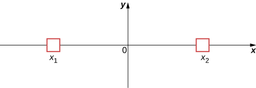
To illustrate this interpretation, consider the simple case of a particle that can occupy a small container either at $x sub 1$ or $x sub 2$ (Figure 7.6). In classical physics, we assume the particle is located either at $x sub 1$ or $x sub 2$ when the observer is not looking. However, in quantum mechanics, the particle may exist in a state of indefinite position—that is, it may be located at $x sub 1$ and $x sub 2$ when the observer is not looking. The assumption that a particle can only have one value of position (when the observer is not looking) is abandoned. Similar comments can be made of other measurable quantities, such as momentum and energy.

An x y coordinate system is shown with two small boxes drawn on the x axis, one at x sub 1 to the left of the origin and the other at x sub 2 to the right of the origin. — **Figure 7.6** A two-state system of position of a particle.

The bizarre consequences of the Copenhagen interpretation of quantum mechanics are illustrated by a creative thought experiment first articulated by Erwin Schrödinger (National Geographic, 2013) (Figure 7.7):

“A cat is placed in a steel box along with a Geiger counter, a vial of poison, a hammer, and a radioactive substance. When the radioactive substance decays, the Geiger detects it and triggers the hammer to release the poison, which subsequently kills the cat. The radioactive decay is a random [probabilistic] process, and there is no way to predict when it will happen. Physicists say the atom exists in a state known as a superposition—both decayed and not decayed at the same time. Until the box is opened, an observer doesn’t know whether the cat is alive or dead—because the cat’s fate is intrinsically tied to whether or not the atom has decayed and the cat would [according to the Copenhagen interpretation] be “living and dead... in equal parts” until it is observed.”

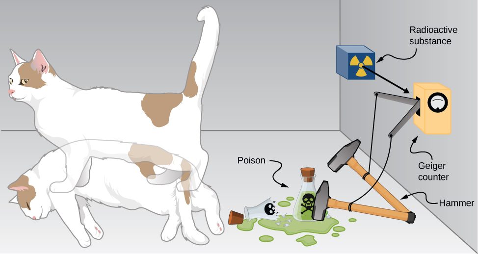
The Schodinger cat thought experiment, consisting of a Geiger counter, a vial of poison, a hammer, a radioactive substance, and a cat is illustrated. Each is shown in two states: The Geiger counter triggered and untriggered, the hammer up and down, the poison vial whole and broken, and the cat alive and dead. — **Figure 7.7** Schrödinger’s cat.

Schrödinger took the absurd implications of this thought experiment (a cat simultaneously dead and alive) as an argument against the Copenhagen interpretation. However, this interpretation remains the most commonly taught view of quantum mechanics.

Two-state systems (left and right, atom decays and does not decay, and so on) are often used to illustrate the principles of quantum mechanics. These systems find many applications in nature, including electron spin and mixed states of particles, atoms, and even molecules. Two-state systems are also finding application in the quantum computer, as mentioned in the introduction of this chapter. Unlike a digital computer, which encodes information in binary digits (zeroes and ones), a quantum computer stores and manipulates data in the form of quantum bits, or qubits. In general, a qubit is not in a state of zero or one, but rather in a mixed state of zero and one. If a large number of qubits are placed in the same quantum state, the measurement of an individual qubit would produce a zero with a probability p, and a one with a probability $q = 1 - p .$ Many scientists believe that quantum computers are the future of the computer industry.

Complex Conjugates

Later in this section, you will see how to use the wave function to describe particles that are “free” or bound by forces to other particles. The specific form of the wave function depends on the details of the physical system. A peculiarity of quantum theory is that these functions are usually complex functions. A complex function is one that contains one or more imaginary numbers $(i = \sqrt{−1})$ . Experimental measurements produce real (nonimaginary) numbers only, so the above procedure to use the wave function must be slightly modified. In general, the probability that a particle is found in the narrow interval (x, x + dx) at time t is given by

$P (x, x + d x) = | Ψ (x, t) |^{2} d x = Ψ^{*} (x, t) Ψ (x, t) d x,$

where $Ψ to the power * open parenthesis x, t close parenthesis$ is the complex conjugate of the wave function. The complex conjugate of a function is obtaining by replacing every occurrence of $i = \sqrt{−1}$ in that function with $− i$ . This procedure eliminates complex numbers in all predictions because the product $Ψ to the power * open parenthesis x, t close parenthesis Ψ open parenthesis x, t close parenthesis$ is always a real number.

Consider the motion of a free particle that moves along the x-direction. As the name suggests, a free particle experiences no forces and so moves with a constant velocity. As we will see in a later section of this chapter, a formal quantum mechanical treatment of a free particle indicates that its wave function has real and complex parts. In particular, the wave function is given by

$Ψ (x, t) = A cos (k x - ω t) + i A sin (k x - ω t),$

where A is the amplitude, k is the wave number, and $ω$ is the angular frequency. Using Euler’s formula, $e^{i ϕ} = cos (ϕ) + i sin (ϕ),$ this equation can be written in the form

$Ψ (x, t) = A e^{i (k x - ω t)} = A e^{i ϕ},$

where $ϕ$ is the phase angle. If the wave function varies slowly over the interval $Δ x,$ the probability of finding the particle in that interval is

$P (x, x + Δ x) \approx Ψ^{*} (x, t) Ψ (x, t) Δ x = (A e^{i ϕ}) (A^{*} e^{− i ϕ}) Δ x = (A^{*} A) Δ x .$

If A has real and complex parts $(a + i b$ , where a and b are real constants), then

$A^{*} A = (a + i b) (a - i b) = a^{2} + b^{2} .$

Notice that the complex numbers have vanished. Thus,

$P (x, x + Δ x) \approx | A |^{2} Δ x$

is a real quantity. The interpretation of $Ψ to the power * open parenthesis x, t close parenthesis Ψ open parenthesis x, t close parenthesis$ as a probability density ensures that the predictions of quantum mechanics can be checked in the “real world.”

Expectation Values

In classical mechanics, the solution to an equation of motion is a function of a measurable quantity, such as x(t), where x is the position and t is the time. Note that the particle has one value of position for any time t. In quantum mechanics, however, the solution to an equation of motion is a wave function, $Ψ (x, t) .$ The particle has many values of position for any time t, and only the probability density of finding the particle, $| Ψ open parenthesis x, t close parenthesis | squared$ , can be known. The average value of position for a large number of particles with the same wave function is expected to be

$〈 x 〉 = \int_{− \infty}^{\infty} x P (x, t) d x = \int_{− \infty}^{\infty} x Ψ^{*} (x, t) Ψ (x, t) d x .$

This is called the expectation value of the position. It is usually written

$〈 x 〉 = \int_{− \infty}^{\infty} Ψ^{*} (x, t) x Ψ (x, t) d x,$

(7.7)

where the x is sandwiched between the wave functions. The reason for this will become apparent soon. Formally, x is called the position operator.

At this point, it is important to stress that a wave function can be written in terms of other quantities as well, such as velocity (v), momentum (p), and kinetic energy (K). The expectation value of momentum, for example, can be written

$〈 p 〉 = \int_{− \infty}^{\infty} Ψ^{*} (p, t) p Ψ (p, t) d p,$

Where dp is used instead of dx to indicate an infinitesimal interval in momentum. In some cases, we know the wave function in position, $Ψ (x, t),$ but seek the expectation of momentum. The procedure for doing this is

$〈 p 〉 = \int_{− \infty}^{\infty} Ψ^{*} (x, t) (− i ℏ \frac{d}{d x}) Ψ (x, t) d x,$

(7.9)

where the quantity in parentheses, sandwiched between the wave functions, is called the momentum operator in the x-direction. [The momentum operator in Equation 7.9 is said to be the position-space representation of the momentum operator.] The momentum operator must act (operate) on the wave function to the right, and then the result must be multiplied by the complex conjugate of the wave function on the left, before integration. The momentum operator in the x-direction is sometimes denoted

${(p_{x})}_{op} = − i ℏ \frac{d}{d x},$

Momentum operators for the y- and z-directions are defined similarly. This operator and many others are derived in a more advanced course in modern physics. In some cases, this derivation is relatively simple. For example, the kinetic energy operator is just

${(K)}_{op} = \frac{1}{2} m {(v_{x})}_{op}^{2} = \frac{{(p_{x})}_{op}^{2}}{2 m} = \frac{{(− i ℏ \frac{d}{d x})}^{2}}{2 m} = \frac{− ℏ^{2}}{2 m} (\frac{d}{d x}) (\frac{d}{d x}) .$

Thus, if we seek an expectation value of kinetic energy of a particle in one dimension, two successive ordinary derivatives of the wave function are required before integration.

Expectation-value calculations are often simplified by exploiting the symmetry of wave functions. Symmetric wave functions can be even or odd. An even function is a function that satisfies

$ψ (x) = ψ (- x) .$

In contrast, an odd function is a function that satisfies

$ψ (x) = - ψ (- x) .$

An example of even and odd functions is shown in Figure 7.8. An even function is symmetric about the y-axis. This function is produced by reflecting $ψ (x)$ for x > 0 about the vertical y-axis. By comparison, an odd function is generated by reflecting the function about the y-axis and then about the x-axis. (An odd function is also referred to as an anti-symmetric function.)

Two wave functions are plotted as a function of x. The vertical scale runs form -0.5 to +0.5 and the horizontal scale from -4 to 4. The even function is plotted in blue. It is symmetric about the origin, positive for all values of x, and going to zero at the ends. This particular even function has a positive minimum at the origin and maxima on either side. The odd function is zero at the origin and at the ends, negative to the left of the origin, where it has a minimum, and positive to the right, where it has a maximum. The function is antisymmetric, meaning that the negative half is the same shape as the right half, but inverted, that is, generated by reflecting the function about the y-axis and then about the x-axis. — **Figure 7.8** Examples of even and odd wave functions.

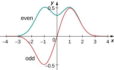
In general, an even function times an even function produces an even function. A simple example of an even function is the product $x squared e to the power − x squared$ (even times even is even). Similarly, an odd function times an odd function produces an even function, such as x sin x (odd times odd is even). However, an odd function times an even function produces an odd function, such as $x e to the power − x squared$ (odd times even is odd). The integral over all space of an odd function is zero, because the total area of the function above the x-axis cancels the (negative) area below it. As the next example shows, this property of odd functions is very useful.

Example 3 Expectation Value (Part I)

The normalized wave function of a particle is

$ψ (x) = e^{− | x | / x_{0}} / \sqrt{x_{0}} .$

Find the expectation value of position.

Strategy Substitute the wave function into Equation 7.7 and evaluate. The position operator introduces a multiplicative factor only, so the position operator need not be “sandwiched.”

Solution First multiply, then integrate:

$〈 x 〉 = \int_{− \infty}^{+ \infty} d x x | ψ (x) |^{2} = {\int_{− \infty}^{+ \infty} d x x | \frac{e^{− | x | / x_{0}}}{\sqrt{x_{0}}} |}^{2} = \frac{1}{x_{0}} \int_{− \infty}^{+ \infty} d x x e^{−2 | x | / x_{0}} = 0 .$

Significance The function in the integrand $open parenthesis x e to the power −2 | x | / x sub 0 close parenthesis$ is odd since it is the product of an odd function (x) and an even function $open parenthesis e to the power −2 | x | / x sub 0 close parenthesis$ . The integral vanishes because the total area of the function about the x-axis cancels the (negative) area below it. The result $open parenthesis 〈 x 〉 equals 0 close parenthesis$ is not surprising since the probability density function is symmetric about $x equals 0$ .

Example 4 Expectation Value (Part II)

The time-dependent wave function of a particle confined to a region between 0 and L is

$ψ (x, t) = A e^{− i ω t} sin (π x / L)$

where $ω$ is angular frequency. (Note: The function varies as a sine because of the limits (0 to L). When $x equals 0,$ the sine factor is zero and the wave function is zero, consistent with the boundary conditions.) Calculate the expectation values of position, momentum, and kinetic energy.

Strategy We must first normalize the wave function to find A. Then we use the operators to calculate the expectation values.

Solution Computation of the normalization constant:

$1 = \int_{0}^{L} d x ψ^{*} (x) ψ (x) = \int_{0}^{L} d x (A e^{+ i ω t} sin \frac{π x}{L}) (A e^{− i ω t} sin \frac{π x}{L}) = A^{2} \int_{0}^{L} d x {sin}^{2} \frac{π x}{L} = A^{2} \frac{L}{2} \Rightarrow A = \sqrt{\frac{2}{L}} .$

The expectation value of position is

$〈 x 〉 = \int_{0}^{L} d x ψ^{*} (x) x ψ (x) = \int_{0}^{L} d x (A e^{+ i ω t} sin \frac{π x}{L}) x (A e^{− i ω t} sin \frac{π x}{L}) = A^{2} \int_{0}^{L} d x x {sin}^{2} \frac{π x}{L} = A^{2} \frac{L^{2}}{4} = \frac{L}{2} .$

The expectation value of momentum in the x-direction also requires an integral. To set this integral up, the associated operator must— by rule—act to the right on the wave function $ψ (x)$ :

$− i ℏ \frac{d}{d x} ψ (x) = − i ℏ \frac{d}{d x} A e^{− i ω t} sin \frac{π x}{L} = − i \frac{A h}{2 L} e^{− i ω t} cos \frac{π x}{L} .$

Therefore, the expectation value of momentum is

$〈 p 〉 = \int_{0}^{L} d x (A e^{+ i ω t} sin \frac{π x}{L}) (− i \frac{A h}{2 L} e^{− i ω t} cos \frac{π x}{L}) = − i \frac{A^{2} h}{4 L} \int_{0}^{L} d x sin \frac{2 π x}{L} = 0 .$

The function in the integral is a sine function with a wavelength equal to the width of the well, L—an odd function about $x equals L / 2$ . As a result, the integral vanishes.

The expectation value of kinetic energy in the x-direction requires the associated operator to act on the wave function:

$- \frac{ℏ^{2}}{2 m} \frac{d^{2}}{d x^{2}} ψ (x) = - \frac{ℏ^{2}}{2 m} \frac{d^{2}}{d x^{2}} A e^{− i ω t} sin \frac{π x}{L} = - \frac{ℏ^{2}}{2 m} A e^{− i ω t} \frac{d^{2}}{d x^{2}} sin \frac{π x}{L} = \frac{A h^{2}}{8 m L^{2}} e^{− i ω t} sin \frac{π x}{L} .$

Thus, the expectation value of the kinetic energy is

$\begin{matrix} 〈 K 〉 & = \int_{0}^{L} d x (A e^{+ i ω t} sin \frac{π x}{L}) (\frac{A h^{2}}{8 m L^{2}} e^{− i ω t} sin \frac{π x}{L}) \\ = \frac{A^{2} h^{2}}{8 m L^{2}} \int_{0}^{L} d x {sin}^{2} \frac{π x}{L} = \frac{A^{2} h^{2}}{8 m L^{2}} \frac{L}{2} = \frac{h^{2}}{8 m L^{2}} . \end{matrix}$

Significance The average position of a large number of particles in this state is L/2. The average momentum of these particles is zero because a given particle is equally likely to be moving right or left. However, the particle is not at rest because its average kinetic energy is not zero. Finally, the probability density is

$| ψ | squared equals open parenthesis 2 / L close parenthesis sin squared open parenthesis π x / L close parenthesis.$

This probability density is largest at location L/2 and is zero at $x equals 0$ and at $x = L .$ Note that these conclusions do not depend explicitly on time.

Quantum mechanics makes many surprising predictions. However, in 1920, Niels Bohr (founder of the Niels Bohr Institute in Copenhagen, from which we get the term “Copenhagen interpretation”) asserted that the predictions of quantum mechanics and classical mechanics must agree for all macroscopic systems, such as orbiting planets, bouncing balls, rocking chairs, and springs. This correspondence principle is now generally accepted. It suggests the rules of classical mechanics are an approximation of the rules of quantum mechanics for systems with very large energies. Quantum mechanics describes both the microscopic and macroscopic world, but classical mechanics describes only the latter.

Summary

In quantum mechanics, the state of a physical system is represented by a wave function.
In Born’s interpretation, the square of the particle’s wave function represents the probability density of finding the particle around a specific location in space.
Wave functions must first be normalized before using them to make predictions.
The expectation value is the average value of a quantity that requires a wave function and an integration.

Conceptual Questions

What is the physical unit of a wave function, $Ψ (x, t) ?$ What is the physical unit of the square of this wave function?

$1 / the square root of L,$ where $L = length$ ; 1/L, where $L = length$

Can the magnitude of a wave function $open parenthesis Ψ to the power * open parenthesis x, t close parenthesis Ψ open parenthesis x, t close parenthesis close parenthesis$ be a negative number? Explain.

What kind of physical quantity does a wave function of an electron represent?

The wave function does not correspond directly to any measured quantity. It is a tool for predicting the values of physical quantities.

What is the physical meaning of a wave function of a particle?

What is the meaning of the expression “expectation value?” Explain.

The average value of the physical quantity for a large number of particles with the same wave function.

Problems

Compute $| Ψ open parenthesis x, t close parenthesis | squared$ for the function $Ψ (x, t) = ψ (x) sin ω t$ , where $ω$ is a real constant.

$| ψ open parenthesis x close parenthesis | squared sin squared ω t$

Given the complex-valued function $f (x, y) = (x - i y) / (x + i y)$ , calculate $| f open parenthesis x, y close parenthesis | squared$ .

Which one of the following functions, and why, qualifies to be a wave function of a particle that can move along the entire real axis? (a) $ψ (x) = A e^{− x^{2}}$ ;
(b) $ψ (x) = A e^{− x}$ ; (c) $ψ (x) = A tan x$ ;
(d) $ψ open parenthesis x close parenthesis equals A open parenthesis sin x close parenthesis / x$ ; (e) $ψ (x) = A e^{− | x |}$ .

(a), (d), and (e) can be normalized

A particle with mass m moving along the x-axis and its quantum state is represented by the following wave function:

$Ψ (x, t) = {\begin{matrix} 0, & x < 0, \\ A x e^{− α x} e^{− i E t / ℏ}, & x \geq 0, \end{matrix}$

where $α = 2.0 \times 10^{10} m^{−1}$ . (a) Find the normalization constant. (b) Find the probability that the particle can be found on the interval $0 less than or equal to x less than or equal to L$ . (c) Find the expectation value of position. (d) Find the expectation value of kinetic energy.

A wave function of a particle with mass m is given by

$ψ (x) = {\begin{matrix} A cos α x, & - \frac{π}{2 α} \leq x \leq + \frac{π}{2 α}, \\ 0, & otherwise, \end{matrix}$

where $α = 1.00 \times 10^{10} / m$ . (a) Find the normalization constant. (b) Find the probability that the particle can be found on the interval $0 \leq x \leq 0.5 \times 10^{−10} m$ . (c) Find the particle’s average position. (d) Find its average momentum. (e) Find its average kinetic energy.

a. $A = \sqrt{2 α / π}$ ; b. $probability equals 29.3 %$ ; c. $〈 x 〉 equals 0$ ; d. $〈 p 〉 equals 0$ ; e. $〈 K 〉 equals α squared ℏ squared / 2 m$