16.1 Angles in Degrees

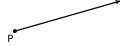
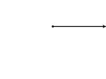
This section serves as a review of the concept of `angle' and the use of the degree system to measure angles. Recall that a ray is usually described as a `half-line' and can be thought of as a line segment in which one of the two endpoints is pushed off infinitely distant from the other, as pictured below. The point from which the ray originates is called the initial point of the ray.

Figure: A ray with initial point . — **Figure 16.1** A ray with initial point $P$ .

When two rays share a common initial point they form an angle and the common initial point is called the vertex of the angle. Two examples of what are commonly thought of as angles are

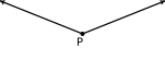
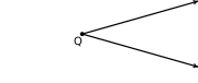
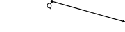
Figure: An angle with vertex . — **Figure 16.2** An angle with vertex $P$ .

However, the two figures below also depict angles - albeit these are, in some sense, extreme cases. In the first case, the two rays are directly opposite each other forming what is known as a straight angle; in the second, the rays are identical so the `angle' is indistinguishable from the ray itself.

Figure: A straight angle. — **Figure 16.4** A straight angle.

Coordinate-plane figure. — **Figure 16.5**

The measure of an angle is a number which indicates the amount of rotation that separates the rays of the angle. There is one immediate problem with this, as pictured below.

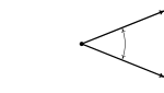
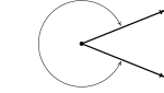
Which amount of rotation are we attempting to quantify? What we have just discovered is that we have at least two angles described by this diagram.¹ Clearly these two angles have different measures because one appears to represent a larger rotation than the other, so we must label them differently. In this book, we use lower case Greek letters such as $α$ (alpha), $β$ (beta), $γ$ (gamma) and $θ$ (theta) to label angles. So, for instance, we have

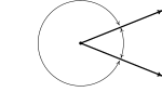
One system to measure angles is degree measure. Quantities measured in degrees are denoted by the symbol ` $∘$ .' One complete revolution as shown below is $360 degrees$ , and parts of a revolution are measured proportionately.² Thus half of a revolution (a straight angle) measures $\frac{1}{2} (360^{\circ}) = 180^{\circ}$ , a quarter of a revolution (a right angle) measures $\frac{1}{4} (360^{\circ}) = 90^{\circ}$ and so on.

Figure: One revolution — **Figure 16.9** One revolution $↔ 360 degrees$

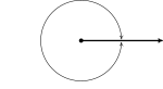
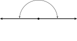
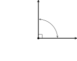
Note that in the above figure, we have used the small square ` $∎$ ' to denote a right angle, as is commonplace in Geometry. Recall that if an angle measures strictly between $0 degrees$ and $90 degrees$ it is called an acute angle and if it measures strictly between $90 degrees$ and $180 degrees$ it is called an obtuse angle. It is important to note that, theoretically, we can know the measure of any angle as long as we know the proportion it represents of entire revolution.³ For instance, the measure of an angle which represents a rotation of $\frac{2}{3}$ of a revolution would measure $\frac{2}{3} (360^{\circ}) = 240^{\circ}$ , the measure of an angle which constitutes only $\frac{1}{12}$ of a revolution measures $\frac{1}{12} (360^{\circ}) = 30^{\circ}$ and an angle which indicates no rotation at all is measured as $0 degrees$ .

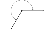
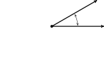
Using our definition of degree measure, we have that $1 degrees$ represents the measure of an angle which constitutes $\frac{1}{360}$ of a revolution. Even though it may be hard to draw, it is nonetheless not difficult to imagine an angle with measure smaller than $1 degrees$ . There are two ways to subdivide degrees. The first, and most familiar, is decimal degrees. For example, an angle with a measure of $30.5 degrees$ would represent a rotation halfway between $30 degrees$ and $31 degrees$ , or equivalently, $\frac{30.5}{360} = \frac{61}{720}$ of a full rotation. This can be taken to the limit using Calculus so that measures like $the square root of 2 degrees$ make sense.⁴ The second way to divide degrees is the Degree - Minute - Second (DMS) system. In this system, one degree is divided equally into sixty minutes, and in turn, each minute is divided equally into sixty seconds.⁵ In symbols, we write $1 degrees equals 60 prime$ and $1 prime equals 60 double prime$ , from which it follows that $1 degrees equals 3600 double prime$ . To convert a measure of $42.125 degrees$ to the DMS system, we start by noting that ${42.125}^{\circ} = 42^{\circ} + {0.125}^{\circ}$ . Converting the partial amount of degrees to minutes, we find ${0.125}^{\circ} (\frac{60^{'}}{1^{\circ}}) = {7.5}^{'} = 7^{'} + {0.5}^{'}$ . Converting the partial amount of minutes to seconds gives ${0.5}^{'} (\frac{60^{''}}{1^{'}}) = 30^{''}$ . Putting it all together yields

$\begin{matrix} {42.125}^{\circ} & = & 42^{\circ} + {0.125}^{\circ} \\ = & 42^{\circ} + {7.5}^{'} \\ = & 42^{\circ} + 7^{'} + {0.5}^{'} \\ = & 42^{\circ} + 7^{'} + 30^{''} \\ = & 42^{\circ} 7^{'} 30^{''} \end{matrix}$

On the other hand, to convert $117 degrees ⁢ 15 prime ⁢ 45 double prime$ to decimal degrees, we first compute $15^{'} (\frac{1^{\circ}}{60^{'}}) = {\frac{1}{4}}^{\circ}$ and $45^{''} (\frac{1^{\circ}}{3600^{''}}) = {\frac{1}{80}}^{\circ}$ . Then we find

$\begin{matrix} 117^{\circ} 15^{'} 45^{''} & = & 117^{\circ} + 15^{'} + 45^{''} \\ = & 117^{\circ} + {\frac{1}{4}}^{\circ} + {\frac{1}{80}}^{\circ} \\ = & {\frac{9381}{80}}^{\circ} \\ = & {117.2625}^{\circ} \end{matrix}$

Recall that two acute angles are called complementary angles if their measures add to $90 degrees$ . Two angles, either a pair of right angles or one acute angle and one obtuse angle, are called supplementary angles if their measures add to $180 degrees$ . In the diagram below, the angles $α$ and $β$ are supplementary angles while the pair $γ$ and $θ$ are complementary angles.

Figure: Supplementary Angles — **Figure 16.15** Supplementary Angles

Figure: Complementary Angles — **Figure 16.16** Complementary Angles

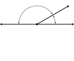
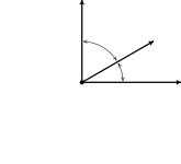
In practice, the distinction between the angle itself and its measure is blurred so that the sentence ` $α$ is an angle measuring $42 degrees$ ' is often abbreviated as ` $α equals 42 degrees$ .' It is now time for an example.

Example 1

Let $α equals 111.371 degrees$ and $β equals 37 degrees ⁢ 28 prime ⁢ 17 double prime$ .

Convert $α$ to the DMS system. Round your answer to the nearest second.
Convert $β$ to decimal degrees. Round your answer to the nearest thousandth of a degree.
Sketch $α$ and $β$ .
Find a supplementary angle for $α$ .
Find a complementary angle for $β$ .

To convert $α$ to the DMS system, we start with ${111.371}^{\circ} = 111^{\circ} + {0.371}^{\circ}$ . Next we convert ${0.371}^{\circ} (\frac{60^{'}}{1^{\circ}}) = {22.26}^{'}$ . Writing ${22.26}^{'} = 22^{'} + {0.26}^{'}$ , we convert ${0.26}^{'} (\frac{60^{''}}{1^{'}}) = {15.6}^{''}$ . Hence,
$\begin{matrix} {111.371}^{\circ} & = & 111^{\circ} + {0.371}^{\circ} \\ = & 111^{\circ} + {22.26}^{'} \\ = & 111^{\circ} + 22^{'} + {0.26}^{'} \\ = & 111^{\circ} + 22^{'} + {15.6}^{''} \\ = & 111^{\circ} 22^{'} {15.6}^{''} \end{matrix}$
Rounding to seconds, we obtain $α approximately equals 111 degrees ⁢ 22 prime ⁢ 16 double prime$ .
To convert $β$ to decimal degrees, we convert $28^{'} (\frac{1^{\circ}}{60^{'}}) = {\frac{7}{15}}^{\circ}$ and $17^{''} (\frac{1^{\circ}}{3600^{'}}) = {\frac{17}{3600}}^{\circ}$ . Putting it all together, we have
$\begin{matrix} 37^{\circ} 28^{'} 17^{''} & = & 37^{\circ} + 28^{'} + 17^{''} \\ = & 37^{\circ} + {\frac{7}{15}}^{\circ} + {\frac{17}{3600}}^{\circ} \\ = & {\frac{134897}{3600}}^{\circ} \\ \approx & {37.471}^{\circ} \end{matrix}$
To sketch $α$ , we first note that $90 degrees less than α less than 180 degrees$ . Dividing this range in half, we get $90 degrees less than α less than 135 degrees$ , and once more, we have $90 degrees less than α less than 112.5 degrees$ . This gives us a pretty good estimate for $α$ , as shown below.⁶ Proceeding similarly for $β$ , we find $0 degrees less than β less than 90 degrees$ , then $0 degrees less than β less than 45 degrees$ , $22.5 degrees less than β less than 45 degrees$ , and lastly, $33.75 degrees less than β less than 45 degrees$ .
Figure 16.17 Angle $α$
Figure 16.18 Angle $β$
To find a supplementary angle for $α$ , we seek an angle $θ$ so that $α + θ = 180^{\circ}$ . We get $θ = 180^{\circ} - α = 180^{\circ} - {111.371}^{\circ} = {68.629}^{\circ}$ .
To find a complementary angle for $β$ , we seek an angle $γ$ so that $β + γ = 90^{\circ}$ . We get $γ = 90^{\circ} - β = 90^{\circ} - 37^{\circ} 28^{'} 17^{''}$ . While we could reach for the calculator to obtain an approximate answer, we choose instead to do a bit of sexagesimal⁷ arithmetic. We first rewrite $90^{\circ} = 90^{\circ} 0^{'} 0^{''} = 89^{\circ} 60^{'} 0^{''} = 89^{\circ} 59^{'} 60^{''}$ . In essence, we are `borrowing' $1 degrees equals 60 prime$ from the degree place, and then borrowing $1 prime equals 60 double prime$ from the minutes place.⁸ This yields, $γ = 90^{\circ} - 37^{\circ} 28^{'} 17^{''} = 89^{\circ} 59^{'} 60^{''} - 37^{\circ} 28^{'} 17^{''} = 52^{\circ} 31^{'} 43^{''}$ .

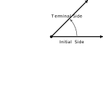
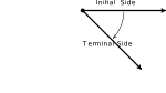
Up to this point, we have discussed only angles which measure between $0 degrees$ and $360 degrees$ , inclusive. Ultimately, we want to use the arsenal of Algebra which we have stockpiled in Chapters 1 through 10 to not only solve geometric problems involving angles, but also to extend their applicability to other real-world phenomena. A first step in this direction is to extend our notion of `angle' from merely measuring an extent of rotation to quantities which indicate an amount of rotation along with a direction. To that end, we introduce the concept of an oriented angle. As its name suggests, in an oriented angle, the direction of the rotation is important. We imagine the angle being swept out starting from an initial side and ending at a terminal side, as shown below. When the rotation is counter-clockwise⁹ from initial side to terminal side, we say that the angle is positive; when the rotation is clockwise, we say that the angle is negative.

$A positive angle, 45 degrees$

$A negative angle, - 45^{\circ}$

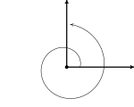
At this point, we also extend our allowable rotations to include angles which encompass more than one revolution. For example, to sketch an angle with measure $450 degrees$ we start with an initial side, rotate counter-clockwise one complete revolution (to take care of the `first' $360 degrees$ ) then continue with an additional $90 degrees$ counter-clockwise rotation, as seen below.

To further connect angles with the Algebra which has come before, we shall often overlay an angle diagram on the coordinate plane. An angle is said to be in standard position if its vertex is the origin and its initial side coincides with the positive horizontal (usually labeled as the $x$ -) axis. Angles in standard position are classified according to where their terminal side lies. For instance, an angle in standard position whose terminal side lies in Quadrant I is called a `Quadrant I angle'. If the terminal side of an angle lies on one of the coordinate axes, it is called a quadrantal angle. Two angles in standard position are called coterminal if they share the same terminal side.¹⁰ In the figure below, $α equals 120 degrees$ and $β = - 240^{\circ}$ are two coterminal Quadrant II angles drawn in standard position. Note that $α = β + 360^{\circ}$ , or equivalently, $β = α - 360^{\circ}$ . We leave it as an exercise to the reader to verify that coterminal angles always differ by a multiple of $360 degrees$ .¹¹ More precisely, if $α$ and $β$ are coterminal angles, then $β = α + 360^{\circ} \cdot k$ where $k$ is an integer.¹²

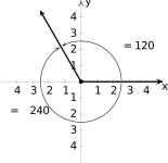
Two coterminal angles, $α equals 120 degrees$ and $β = - 240^{\circ}$ , in standard position.

Example 2

Graph each of the (oriented) angles below in standard position and classify them according to where their terminal side lies. Find three coterminal angles, at least one of which is positive and one of which is negative.

$α equals 60 degrees$
$β = - 225^{\circ}$
$γ equals 540 degrees$
$ϕ = - 750^{\circ}$

To graph $α equals 60 degrees$ , we draw an angle with its initial side on the positive $x$ -axis and rotate counter-clockwise $\frac{60^{\circ}}{360^{\circ}} = \frac{1}{6}$ of a revolution. We see that $α$ is a Quadrant I angle. To find angles which are coterminal, we look for angles $θ$ of the form $θ = α + 360^{\circ} \cdot k$ , for some integer $k$ . When $k equals 1$ , we get $θ = 60^{\circ} + 360^{\circ} = 420^{\circ}$ . Substituting $k = - 1$ gives $θ = 60^{\circ} - 360^{\circ} = - 300^{\circ}$ . Finally, if we let $k equals 2$ , we get $θ = 60^{\circ} + 720^{\circ} = 780^{\circ}$ .
Since $β = - 225^{\circ}$ is negative, we start at the positive $x$ -axis and rotate clockwise $\frac{225^{\circ}}{360^{\circ}} = \frac{5}{8}$ of a revolution. We see that $β$ is a Quadrant II angle. To find coterminal angles, we proceed as before and compute $θ = - 225^{\circ} + 360^{\circ} \cdot k$ for integer values of $k$ . We find $135 degrees$ , $minus 585 degrees$ and $495 degrees$ are all coterminal with $minus 225 degrees$ .
Figure 16.23
Figure 16.24
$α equals 60 degrees$ in standard position.
$β = - 225^{\circ}$ in standard position.
Since $γ equals 540 degrees$ is positive, we rotate counter-clockwise from the positive $x$ -axis. One full revolution accounts for $360 degrees$ , with $180 degrees$ , or $\frac{1}{2}$ of a revolution remaining. Since the terminal side of $γ$ lies on the negative $x$ -axis, $γ$ is a quadrantal angle. All angles coterminal with $γ$ are of the form $θ = 540^{\circ} + 360^{\circ} \cdot k$ , where $k$ is an integer. Working through the arithmetic, we find three such angles: $180 degrees$ , $minus 180 degrees$ and $900 degrees$ .
The Greek letter $ϕ$ is pronounced `fee' or `fie' and since $ϕ$ is negative, we begin our rotation clockwise from the positive $x$ -axis. Two full revolutions account for $720 degrees$ , with just $30 degrees$ or $\frac{1}{12}$ of a revolution to go. We find that $ϕ$ is a Quadrant IV angle. To find coterminal angles, we compute $θ = - 750^{\circ} + 360^{\circ} \cdot k$ for a few integers $k$ and obtain $minus 390 degrees$ , $minus 30 degrees$ and $330 degrees$ .
Figure 16.25
Figure 16.26
$γ equals 540 degrees$ in standard position.
$ϕ = - 750^{\circ}$ in standard position.

Note that since there are infinitely many integers, any given angle has infinitely many coterminal angles, and the reader is encouraged to plot the few sets of coterminal angles found in Example B.1.2 to see this.

As we'll see in Section B.2 and throughout Chapter 13, degree measure is very popular for many applications involving geometry and modeling physical forces. In Section 11.1, we'll introduce a different method of measuring angles, radian measure, which is tied directly to arc length and is useful in other applications involving circular motion and periodic phenomenon.

Exercises

In Exercises -, convert the angles into the DMS system. Round each of your answers to the nearest second.

$63.75 degrees$
$200.325 degrees$
$minus 317.06 degrees$
$179.999 degrees$

In Exercises -, convert the angles into decimal degrees. Round each of your answers to three decimal places.

$125 degrees ⁢ 50 prime$
$minus 32 degrees ⁢ 10 prime ⁢ 12 double prime$
$502 degrees ⁢ 35 prime$
$237 degrees ⁢ 58 prime ⁢ 43 double prime$

In Exercises -, graph the oriented angle in standard position. Classify each angle according to where its terminal side lies and then give two coterminal angles, one of which is positive and the other negative.

$30 degrees$
$120 degrees$
$225 degrees$
$330 degrees$
$minus 30 degrees$
$minus 135 degrees$
$minus 240 degrees$
$minus 270 degrees$
$405 degrees$
$840 degrees$
$minus 510 degrees$
$minus 900 degrees$
With help from your classmates, explain why if $(x, y)$ is a point on the terminal side of an angle $α$ in standard position, then so is $(r x, r y)$ for any number $r greater than 0$ . What happens if $r less than 0$ ?

Answers

$63 degrees ⁢ 45 prime$
$200 degrees ⁢ 19 prime ⁢ 30 double prime$
$minus 317 degrees ⁢ 3 prime ⁢ 36 double prime$
$179 degrees ⁢ 59 prime ⁢ 56 double prime$
$125.833 degrees$
$minus 32.17 degrees$
$502.583 degrees$
$237.979 degrees$
$30 degrees$ is a Quadrant I angle coterminal with $390 degrees$ and $minus 330 degrees$
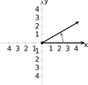
Figure 16.27
$120 degrees$ is a Quadrant II angle coterminal with $480 degrees$ and $minus 240 degrees$
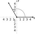
Figure 16.28
$225 degrees$ is a Quadrant III angle coterminal with $585 degrees$ and $minus 135 degrees$
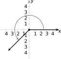
Figure 16.29
$330 degrees$ is a Quadrant IV angle coterminal with $690 degrees$ and $minus 30 degrees$
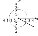
Figure 16.30
$minus 30 degrees$ is a Quadrant IV angle coterminal with $330 degrees$ and $minus 390 degrees$
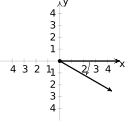
Figure 16.31
$minus 135 degrees$ is a Quadrant III angle coterminal with $225 degrees$ and $minus 495 degrees$
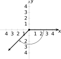
Figure 16.32
$minus 240 degrees$ is a Quadrant II angle coterminal with $120 degrees$ and $minus 600 degrees$
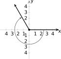
Figure 16.33
$minus 270 degrees$ is a quadrantal angle coterminal with $90 degrees$ and $minus 630 degrees$
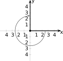
Figure 16.34
$405 degrees$ is a Quadrant I angle coterminal with $45 degrees$ and $minus 315 degrees$
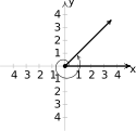
Figure 16.35
$840 degrees$ is a Quadrant II angle coterminal with $120 degrees$ and $minus 240 degrees$
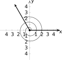
Figure 16.36
$minus 510 degrees$ is a Quadrant III angle coterminal with $minus 150 degrees$ and $210 degrees$
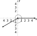
Figure 16.37
$minus 900 degrees$ is a quadrantal angle coterminal with $minus 180 degrees$ and $180 degrees$
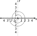
Figure 16.38

The phrase `at least' will be justified in short order. ↩
The choice of ` $360$ ' is most often attributed to the Babylonians . ↩
This is how a protractor is graded. ↩
Awesome math pun aside, this is the same idea behind defining irrational exponents in Section 4.2. ↩
Does this kind of system seem familiar? ↩
If this process seems hauntingly familiar, it should. Compare this method to the Bisection Method introduced in Section 2.3.3. ↩
Like `latus rectum,' this is also a real math term. ↩
This is the exact same kind of `borrowing' you used to do in Elementary School when trying to find $300 minus 125$ . Back then, you were working in a base ten system; here, it is base sixty. ↩
`widdershins' ↩
Note that by being in standard position they automatically share the same initial side which is the positive $x$ -axis. ↩
It is worth noting that all of the pathologies of Analytic Trigonometry result from this innocuous fact. ↩
Recall that this means $k = 0, \pm 1, \pm 2, \dots$ . ↩

Adapted from Precalculus, Preliminary 4th Edition (integrated calculus), by Carl Stitz and Jeff Zeager (stitz-zeager.com), licensed under CC BY-NC-SA 3.0. Changes were made: reformatted as an accessible XYZ web edition. License: CC-BY-NC-SA-3.0.