12.4 Equations and Inequalities Involving the Circular Functions

In Sections 11.2, 11.4 and most recently 12.3, we solved some basic equations involving the trigonometric functions. Below we summarize the techniques we've employed thus far. Note that we use the neutral letter ` $u$ ' as the argument of each circular function for generality.

Strategies for Solving Basic Equations Involving the Circular Functions

To solve $\cos (u) = c$ or $\sin (u) = c$ for $minus 1 less than or equal to c less than or equal to 1$ , first solve for $u$ in the interval $open bracket 0, 2 ⁢ π close parenthesis$ and add integer multiples of the period $2 ⁢ π$ . If $c less than minus 1$ or of $c greater than 1$ , there are no real solutions.
To solve $\sec (u) = c$ or $\csc (u) = c$ for $c less than or equal to minus 1$ or $c greater than or equal to 1$ , convert to cosine or sine, respectively, and solve as above. If $minus 1 less than c less than 1$ , there are no real solutions.
To solve $\tan (u) = c$ for any real number $c$ , first solve for $u$ in the interval $(- \frac{π}{2}, \frac{π}{2})$ and add integer multiples of the period $π$ .
To solve $\cot (u) = c$ for $c not equal to 0$ , convert to tangent and solve as above. If $c equals 0$ , the solution to $cot ⁡ open parenthesis u close parenthesis equals 0$ is $u = \frac{π}{2} + π k$ for integers $k$ .

Using the above guidelines, we can comfortably solve $\sin (x) = \frac{1}{2}$ and find the solution $x = \frac{π}{6} + 2 π k$ or $x = \frac{5 π}{6} + 2 π k$ for integers $k$ . But how do we solve the related equation $\sin (3 x) = \frac{1}{2}$ ?

Since this equation has the form $\sin (u) = \frac{1}{2}$ , we know the solutions take the form $u = \frac{π}{6} + 2 π k$ or $u = \frac{5 π}{6} + 2 π k$ for integers $k$ . Since the argument of sine here is $3 ⁢ x$ , we have $3 x = \frac{π}{6} + 2 π k$ or $3 x = \frac{5 π}{6} + 2 π k$ .

To solve for $x$ , we divide both sides¹ of these equations by $3$ , and obtain $x = \frac{π}{18} + \frac{2 π}{3} k$ or $x = \frac{5 π}{18} + \frac{2 π}{3} k$ for integers $k$ . This is the technique employed in the example below.

Example 1

Solve the following equations and check your answers analytically. List the solutions which lie in the interval $open bracket 0, 2 ⁢ π close parenthesis$ and verify them using a graphing utility.

$\cos (2 θ) = - \frac{\sqrt{3}}{2}$
$\csc (\frac{1}{3} θ - π) = \sqrt{2}$
$cot ⁡ open parenthesis 3 ⁢ t close parenthesis equals 0$
$sec squared ⁡ open parenthesis t close parenthesis equals 4$
$\tan (\frac{x}{2}) = - 3$
$sin ⁡ open parenthesis 2 ⁢ x close parenthesis equals 0.87$

The solutions to $\cos (u) = - \frac{\sqrt{3}}{2}$ are $u = \frac{5 π}{6} + 2 π k$ or $u = \frac{7 π}{6} + 2 π k$ for integers $k$ .
Since the argument of cosine here is $2 ⁢ θ$ , this means $2 θ = \frac{5 π}{6} + 2 π k$ or $2 θ = \frac{7 π}{6} + 2 π k$ for integers $k$ . Solving for $θ$ gives $θ = \frac{5 π}{12} + π k$ or $θ = \frac{7 π}{12} + π k$ for integers $k$ .
To check these answers analytically, we substitute them into the original equation. For any integer $k$ :
$\begin{matrix} \cos (2 [\frac{5 π}{12} + π k]) & = & \cos (\frac{5 π}{6} + 2 π k) \\ = & \cos (\frac{5 π}{6}) & (the period of cosine is 2 π) \\ = & - \frac{\sqrt{3}}{2} \end{matrix}$
Similarly, we find $\cos (2 [\frac{7 π}{12} + π k]) = \cos (\frac{7 π}{6} + 2 π k) = \cos (\frac{7 π}{6}) = - \frac{\sqrt{3}}{2}$ .
To determine which of our solutions lie in $open bracket 0, 2 ⁢ π close parenthesis$ , we substitute integer values for $k$ . The solutions we keep come from the values of $k equals 0$ and $k equals 1$ and are $θ = \frac{5 π}{12}$ , $\frac{7 π}{12}$ , $\frac{17 π}{12}$ and $\frac{19 π}{12}$ .
Using a calculator, we graph $y equals cos ⁡ open parenthesis 2 ⁢ θ close parenthesis$ and $y = - \frac{\sqrt{3}}{2}$ over $open bracket 0, 2 ⁢ π close parenthesis$ and examine where these two graphs intersect to verify our answers.
Figure 12.56
$y equals cos ⁡ open parenthesis 2 ⁢ θ close parenthesis$ and $y = - \frac{\sqrt{3}}{2}$
Since this equation has the form $\csc (u) = \sqrt{2}$ , we rewrite this as $\sin (u) = \frac{\sqrt{2}}{2}$ and find $u = \frac{π}{4} + 2 π k$ or $u = \frac{3 π}{4} + 2 π k$ for integers $k$ .
Since the argument of cosecant here is $(\frac{1}{3} θ - π)$ , $\frac{1}{3} θ - π = \frac{π}{4} + 2 π k$ or $\frac{1}{3} θ - π = \frac{3 π}{4} + 2 π k$ .
To solve $\frac{1}{3} θ - π = \frac{π}{4} + 2 π k$ , we first add $π$ to both sides to get $\frac{1}{3} θ = \frac{π}{4} + 2 π k + π$ . A common error is to treat the ` $2 ⁢ π ⁢ k$ ' and ` $π$ ' terms as `like' terms and try to combine them when they are not.
We can, however, combine the ` $π$ ' and ` $\frac{π}{4}$ ' terms to get $\frac{1}{3} θ = \frac{5 π}{4} + 2 π k$ .
We now finish by multiplying both sides by $3$ to get $θ = 3 (\frac{5 π}{4} + 2 π k) = \frac{15 π}{4} + 6 π k$ , where $k$ , as always, runs through the integers.
Solving the other equation, $\frac{1}{3} θ - π = \frac{3 π}{4} + 2 π k$ produces $θ = \frac{21 π}{4} + 6 π k$ for integers $k$ . To check the first family of answers, we substitute, combine line terms, and simplify.
$\begin{matrix} \csc (\frac{1}{3} [\frac{15 π}{4} + 6 π k] - π) & = & \csc (\frac{5 π}{4} + 2 π k - π) \\ = & \csc (\frac{π}{4} + 2 π k) \\ = & \csc (\frac{π}{4}) & (the period of cosecant is 2 π) \\ = & \sqrt{2} \end{matrix}$
The family $θ = \frac{21 π}{4} + 6 π k$ checks similarly.
Despite having infinitely many solutions, we find that none of them lie in $open bracket 0, 2 ⁢ π close parenthesis$ .
To verify this graphically, we check that $y = \csc (\frac{1}{3} θ - π)$ and $y = \sqrt{2}$ do not intersect at all over the interval $open bracket 0, 2 ⁢ π close parenthesis$ .
Figure 12.57
$y = \csc (\frac{1}{3} θ - π)$ and $y = \sqrt{2}$
Since $cot ⁡ open parenthesis 3 ⁢ t close parenthesis equals 0$ has the form $cot ⁡ open parenthesis u close parenthesis equals 0$ , we know $u = \frac{π}{2} + π k$ , so, in this case, $3 t = \frac{π}{2} + π k$ for integers $k$ .
Solving for $t$ yields $t = \frac{π}{6} + \frac{π}{3} k$ . Checking our answers, we get
$\begin{matrix} \cot (3 [\frac{π}{6} + \frac{π}{3} k]) & = & \cot (\frac{π}{2} + π k) \\ = & \cot (\frac{π}{2}) & (the period of cotangent is π) \\ = & 0 \end{matrix}$
As $k$ runs through the integers, we obtain six answers, corresponding to $k equals 0$ through $k equals 5$ , which lie in $open bracket 0, 2 ⁢ π close parenthesis$ : $x = \frac{π}{6}$ , $\frac{π}{2}$ , $\frac{5 π}{6}$ , $\frac{7 π}{6}$ , $\frac{3 π}{2}$ and $\frac{11 π}{6}$ .
Graphing $y equals cot ⁡ open parenthesis 3 ⁢ t close parenthesis$ and $y equals 0$ (the $t$ -axis), we confirm our result.²
Figure 12.58
$y equals cot ⁡ open parenthesis 3 ⁢ t close parenthesis$ and $y equals 0$
The complication in solving an equation like $sec squared ⁡ open parenthesis t close parenthesis equals 4$ comes not from the argument of secant, which is just $t$ , but rather, the fact the secant is being squared: $\sec^{2} (t) = {(\sec (t))}^{2} = 4$ .
To get this equation to look like one of the forms listed on page 12.4, we extract square roots to get $\sec (t) = \pm 2$ . Converting to cosines, we have $\cos (t) = \pm \frac{1}{2}$ .
For $\cos (t) = \frac{1}{2}$ , we get $t = \frac{π}{3} + 2 π k$ or $t = \frac{5 π}{3} + 2 π k$ for integers $k$ . For $\cos (t) = - \frac{1}{2}$ , we get $t = \frac{2 π}{3} + 2 π k$ or $t = \frac{4 π}{3} + 2 π k$ for integers $k$ .
If we take a step back and think of these families of solutions geometrically, we see we are finding the measures of all angles with a reference angle of $\frac{π}{3}$ . As a result, these solutions can be combined and we may write our solutions as $t = \frac{π}{3} + π k$ and $t = \frac{2 π}{3} + π k$ for integers $k$ .
To check the first family of solutions, we note that, depending on the integer $k$ , $\sec (\frac{π}{3} + π k)$ doesn't always equal $\sec (\frac{π}{3})$ . It is true, though, that for all integers $k$ , $\sec (\frac{π}{3} + π k) = \pm \sec (\frac{π}{3}) = \pm 2$ . (Can you show this?) Hence, checking our first family of solutions gives:
$\begin{matrix} \sec^{2} (\frac{π}{3} + π k) & = & {(\pm \sec (\frac{π}{3}))}^{2} \\ = & {(\pm 2)}^{2} \\ = & 4 \end{matrix}$
The check for the family of solutions $t = \frac{2 π}{3} + π k$ is similar.
The solutions which lie in $open bracket 0, 2 ⁢ π close parenthesis$ come from the values $k equals 0$ and $k equals 1$ , namely $t = \frac{π}{3}$ , $\frac{2 π}{3}$ , $\frac{4 π}{3}$ and $\frac{5 π}{3}$ . Graphing $y = {(\sec (t))}^{2}$ and $y equals 4$ confirms our results.
Figure 12.59
$y = {(\sec (t))}^{2}$ and $y equals 4$
The equation $\tan (\frac{x}{2}) = - 3$ has the form $\tan (u) = - 3$ , whose solution is $u = \arctan (- 3) + π k$ .
Hence, $\frac{x}{2} = \arctan (- 3) + π k$ , so $x = 2 \arctan (- 3) + 2 π k$ for integers $k$ . To check, we note

To determine which of our answers lie in the interval $open bracket 0, 2 ⁢ π close parenthesis$ , we first need to get an idea of the value of $2 ⁢ arctan ⁡ open parenthesis minus 3 close parenthesis$ . While we could easily find an approximation using a calculator,³ we proceed analytically, as is our custom.
To get started, we note that since $minus 3 less than 0$ , it $- \frac{π}{2} < \arctan (- 3) < 0$ . Hence, $- π < 2 \arctan (- 3) < 0$ . With regard to our solutions, $x = 2 \arctan (- 3) + 2 π k$ , we see for $k equals 0$ , we get $x = 2 \arctan (- 3) < 0$ , so we discard this answer and all answers $x = 2 \arctan (- 3) + 2 π k$ where $k less than 0$ .
Next, we turn our attention to $k equals 1$ and get $x = 2 \arctan (- 3) + 2 π$ . Starting with the inequality $- π < 2 \arctan (- 3) < 0$ , we add through $2 ⁢ π$ and get $π < 2 \arctan (- 3) + 2 π < 2 π$ . This means $x = 2 \arctan (- 3) + 2 π$ lies in $open bracket 0, 2 ⁢ π close parenthesis$ .
Advancing $k$ to $2$ produces $x = 2 \arctan (- 3) + 4 π$ . Once again, we get from $- π < 2 \arctan (- 3) < 0$ that $3 π < 2 \arctan (- 3) + 4 π < 4 π$ . Since this is outside the interval of interest, $open bracket 0, 2 ⁢ π close parenthesis$ , we discard $x = 2 \arctan (- 3) + 4 π$ and all solutions of the form $x = 2 \arctan (- 3) + 2 π k$ for $k greater than 2$ .
Graphically, $y = \tan (\frac{x}{2})$ and $y = - 3$ intersect only once on $open bracket 0, 2 ⁢ π close parenthesis$ at $x = 2 \arctan (- 3) + 2 π \approx 3.785$ .
Figure 12.60
$y = \tan (\frac{x}{2})$ and $y = - 3$
To solve $sin ⁡ open parenthesis 2 ⁢ x close parenthesis equals 0.87$ , we first note that it has the form $sin ⁡ open parenthesis u close parenthesis equals 0.87$ , which has the family of solutions $u = \arcsin (0.87) + 2 π k$ or $u = π - \arcsin (0.87) + 2 π k$ for integers $k$ .
Since the argument of sine here is $2 ⁢ x$ , we get $2 x = \arcsin (0.87) + 2 π k$ or $2 x = π - \arcsin (0.87) + 2 π k$ which gives $x = \frac{1}{2} \arcsin (0.87) + π k$ or $x = \frac{π}{2} - \frac{1}{2} \arcsin (0.87) + π k$ for integers $k$ . To check,

For the family $x = \frac{π}{2} - \frac{1}{2} \arcsin (0.87) + π k$ , we get

To determine which of these solutions lie in $open bracket 0, 2 ⁢ π close parenthesis$ , we first need to get an idea of the value of $x = \frac{1}{2} \arcsin (0.87)$ . Once again, we could use the calculator, but we adopt an analytic route here.
By definition, $0 < \arcsin (0.87) < \frac{π}{2}$ so that multiplying through by $\frac{1}{2}$ gives us $0 < \frac{1}{2} \arcsin (0.87) < \frac{π}{4}$ .
Starting with the family of solutions $x = \frac{1}{2} \arcsin (0.87) + π k$ , we use the same kind of arguments as in our solution to number above and find only the solutions corresponding to $k equals 0$ and $k equals 1$ lie in $open bracket 0, 2 ⁢ π close parenthesis$ : $x = \frac{1}{2} \arcsin (0.87)$ and $x = \frac{1}{2} \arcsin (0.87) + π$ .
Next, we move to the family $x = \frac{π}{2} - \frac{1}{2} \arcsin (0.87) + π k$ for integers $k$ . Here, we need to get a better estimate of $\frac{π}{2} - \frac{1}{2} \arcsin (0.87)$ . From the inequality $0 < \frac{1}{2} \arcsin (0.87) < \frac{π}{4}$ , we first multiply through by $minus 1$ and then add $\frac{π}{2}$ to get $\frac{π}{2} > \frac{π}{2} - \frac{1}{2} \arcsin (0.87) > \frac{π}{4}$ , or $\frac{π}{4} < \frac{π}{2} - \frac{1}{2} \arcsin (0.87) < \frac{π}{2}$ .
Proceeding with the usual arguments, we find the only solutions which lie in $open bracket 0, 2 ⁢ π close parenthesis$ correspond to $k equals 0$ and $k equals 1$ , namely $x = \frac{π}{2} - \frac{1}{2} \arcsin (0.87)$ and $x = \frac{3 π}{2} - \frac{1}{2} \arcsin (0.87)$ .
All told, we have found four solutions to $sin ⁡ open parenthesis 2 ⁢ x close parenthesis equals 0.87$ in $open bracket 0, 2 ⁢ π close parenthesis$ : $x = \frac{1}{2} \arcsin (0.87) \approx 0.528$ , $x = \frac{1}{2} \arcsin (0.87) + π \approx 3.669$ , $x = \frac{π}{2} - \frac{1}{2} \arcsin (0.87) \approx 1.043$ and $x = \frac{3 π}{2} - \frac{1}{2} \arcsin (0.87) \approx 4.185$ . By graphing $y equals sin ⁡ open parenthesis 2 ⁢ x close parenthesis$ and $y equals 0.87$ , we confirm our results.
Figure 12.61
$y equals sin ⁡ open parenthesis 2 ⁢ x close parenthesis$ and $y equals 0.87$

If one looks closely at the equations and solutions in Example 12.4.1, an interesting relationship evolves between the frequency of the circular function involved in the equation and how many solutions one can expect in the interval $open bracket 0, 2 ⁢ π close parenthesis$ . This relationship is explored in Exercise.

Each of the problems in Example 12.4.1 featured one circular function. If an equation involves two different circular functions or if the equation contains the same circular function but with different arguments, we will need to employ identities and Algebra to reduce the equation to the same form as those given on page 12.4. We demonstrate these techniques in the following example.

Example 2

Solve the following equations and list the solutions which lie in the interval $open bracket 0, 2 ⁢ π close parenthesis$ . Verify your solutions on $open bracket 0, 2 ⁢ π close parenthesis$ graphically.

$3 ⁢ sin cubed ⁡ open parenthesis θ close parenthesis equals sin squared ⁡ open parenthesis θ close parenthesis$
$\sec^{2} (θ) = \tan (θ) + 3$
$\cos (2 t) = 3 \cos (t) - 2$
$\cos (3 t) = 2 - \cos (t)$
$cos ⁡ open parenthesis 3 ⁢ x close parenthesis equals cos ⁡ open parenthesis 5 ⁢ x close parenthesis$
$\sin (2 x) = \sqrt{3} \cos (x)$
$\sin (x) \cos (\frac{x}{2}) + \cos (x) \sin (\frac{x}{2}) = 1$
$\cos (x) - \sqrt{3} \sin (x) = 2$

One approach to solving $3 ⁢ sin cubed ⁡ open parenthesis θ close parenthesis equals sin squared ⁡ open parenthesis θ close parenthesis$ begins with dividing both sides by $\sin^{2} (θ)$ . Doing so, however, assumes that $sin squared ⁡ open parenthesis θ close parenthesis not equal to 0$ which means we risk losing solutions.
Instead, we take a cue from Chapter 2 (since what we have here is a polynomial equation in terms of $\sin (θ)$ ) and gather all the nonzero terms on one side and factor:
$\begin{matrix} 3 \sin^{3} (θ) & = & \sin^{2} (θ) \\ 3 \sin^{3} (θ) - \sin^{2} (θ) & = & 0 \\ \sin^{2} (θ) (3 \sin (θ) - 1) & = & 0 & Factor out \sin^{2} (θ) from both terms. \end{matrix}$
We get $sin squared ⁡ open parenthesis θ close parenthesis equals 0$ or $3 \sin (θ) - 1 = 0$ , so $sin ⁡ open parenthesis θ close parenthesis equals 0$ or $\sin (θ) = \frac{1}{3}$ . The solution to $sin ⁡ open parenthesis θ close parenthesis equals 0$ is $θ = π k$ , with $θ equals 0$ and $θ = π$ being the two solutions which lie in $open bracket 0, 2 ⁢ π close parenthesis$ .
To solve $\sin (θ) = \frac{1}{3}$ , we use the arcsine function to get $θ = \arcsin (\frac{1}{3}) + 2 π k$ or $θ = π - \arcsin (\frac{1}{3}) + 2 π k$ for integers $k$ . We find the two solutions here which lie in $open bracket 0, 2 ⁢ π close parenthesis$ to be $θ = \arcsin (\frac{1}{3}) \approx 0.34$ and $θ = π - \arcsin (\frac{1}{3}) \approx 2.80$ .
To check graphically, we plot $y equals 3 ⁢ open parenthesis sin ⁡ open parenthesis θ close parenthesis close parenthesis cubed$ and $y = {(\sin (θ))}^{2}$ and find the $θ$ -coordinates of the intersection points of these two curves.⁴ (Some extra zooming may be required near $θ equals 0$ and $θ = π$ to verify that these two curves do in fact intersect four times.)
Figure 12.62
$y equals 3 ⁢ open parenthesis sin ⁡ open parenthesis θ close parenthesis close parenthesis cubed$ and $y = {(\sin (θ))}^{2}$
We see immediately in the equation $\sec^{2} (θ) = \tan (θ) + 3$ that there are two different circular functions present, so we look for an identity to express both sides in terms of the same function.
We use the Pythagorean Identity $\sec^{2} (θ) = 1 + \tan^{2} (θ)$ to exchange $\sec^{2} (θ)$ for tangents. What results is a `quadratic in disguise:'⁵
$\begin{matrix} \sec^{2} (θ) & = & \tan (θ) + 3 \\ 1 + \tan^{2} (θ) & = & \tan (θ) + 3 & (Since \sec^{2} (θ) = 1 + \tan^{2} (θ) .) \\ \tan^{2} (θ) - \tan (θ) - 2 & = & 0 \\ u^{2} - u - 2 & = & 0 & Let u = \tan (θ) . \\ (u + 1) (u - 2) & = & 0 \end{matrix}$
This gives $u = - 1$ or $u equals 2$ . Since $u = \tan (θ)$ , we have $\tan (θ) = - 1$ or $tan ⁡ open parenthesis θ close parenthesis equals 2$ .
From $\tan (θ) = - 1$ , we get $θ = - \frac{π}{4} + π k$ for integers $k$ . To solve $tan ⁡ open parenthesis θ close parenthesis equals 2$ , we employ the arctangent function and get $θ = \arctan (2) + π k$ for integers $k$ .
From the first set of solutions, we get $θ = \frac{3 π}{4}$ and $θ = \frac{7 π}{4}$ as our answers which lie in $open bracket 0, 2 ⁢ π close parenthesis$ .
Using the same sort of argument we saw in Example 12.4.1, we get $θ = \arctan (2) \approx 1.107$ and $θ = π + \arctan (2) \approx 4.249$ as answers from our second set of solutions which lie in $open bracket 0, 2 ⁢ π close parenthesis$ .
We verify our solutions below graphically.
Figure 12.63
$y = {(\sec (θ))}^{2}$ and $y = \tan (θ) + 3$
The good news is that in the equation $\cos (2 t) = 3 \cos (t) - 2$ , we have the same circular function, cosine, throughout. The bad news is that we have different arguments, $2 ⁢ t$ and $t$ .
Using the double angle identity $\cos (2 t) = 2 \cos^{2} (t) - 1$ results in another quadratic in disguise:'
$\begin{matrix} \cos (2 t) & = & 3 \cos (t) - 2 \\ 2 \cos^{2} (t) - 1 & = & 3 \cos (t) - 2 & (Since \cos (2 t) = 2 \cos^{2} (t) - 1 .) \\ 2 \cos^{2} (t) - 3 \cos (t) + 1 & = & 0 \\ 2 u^{2} - 3 u + 1 & = & 0 & Let u = \cos (t) . \\ (2 u - 1) (u - 1) & = & 0 \end{matrix}$
We get $u = \frac{1}{2}$ or $u equals 1$ , so $\cos (t) = \frac{1}{2}$ or $cos ⁡ open parenthesis t close parenthesis equals 1$ . Solving $\cos (t) = \frac{1}{2}$ , we get $t = \frac{π}{3} + 2 π k$ or $t = \frac{5 π}{3} + 2 π k$ for integers $k$ . From $cos ⁡ open parenthesis t close parenthesis equals 1$ , we get $t equals 2 ⁢ π ⁢ k$ for integers $k$ .
The answers which lie in $open bracket 0, 2 ⁢ π close parenthesis$ are $t equals 0$ , $\frac{π}{3}$ , and $\frac{5 π}{3}$ . Graphing $y equals cos ⁡ open parenthesis 2 ⁢ t close parenthesis$ and $y = 3 \cos (t) - 2$ , we find that the curves intersect in three places on $open bracket 0, 2 ⁢ π close parenthesis$ and confirm our results.
Figure 12.64
$y equals cos ⁡ open parenthesis 2 ⁢ t close parenthesis$ and $y = 3 \cos (t) - 2$
To solve $\cos (3 t) = 2 - \cos (t)$ , we take a cue from the previous problem and look for an identity to rewrite $cos ⁡ open parenthesis 3 ⁢ t close parenthesis$ in terms of $\cos (t)$ .
From Example 12.2.3, number, we know that $\cos (3 t) = 4 \cos^{3} (t) - 3 \cos (t)$ . This transforms the equation into a polynomial in terms of $\cos (t)$ .
$\begin{matrix} \cos (3 t) & = & 2 - \cos (t) \\ 4 \cos^{3} (t) - 3 \cos (t) & = & 2 - \cos (t) \\ 2 \cos^{3} (t) - 2 \cos (t) - 2 & = & 0 \\ 4 u^{3} - 2 u - 2 & = & 0 & Let u = \cos (t) . \end{matrix}$
Using what we know from Chapter 2, we factor $4 u^{3} - 2 u - 2$ as $(u - 1) (4 u^{2} + 4 u + 2)$ and set each factor equal to $0$ .
We get either $u - 1 = 0$ or $4 u^{2} + 2 u + 2 = 0$ , and since the discriminant of the latter is negative, the only real solution to $4 u^{3} - 2 u - 2 = 0$ is $u equals 1$ .
Since $u = \cos (t)$ , we get $cos ⁡ open parenthesis t close parenthesis equals 1$ , so $t equals 2 ⁢ π ⁢ k$ for integers $k$ . The only solution which lies in $open bracket 0, 2 ⁢ π close parenthesis$ is $t equals 0$ . Our graph below confirms this.
Figure 12.65
$y equals cos ⁡ open parenthesis 3 ⁢ t close parenthesis$ and $y = 2 - \cos (t)$
While we could approach solving the equation $cos ⁡ open parenthesis 3 ⁢ x close parenthesis equals cos ⁡ open parenthesis 5 ⁢ x close parenthesis$ in the same manner as we did the previous two problems, we choose instead to showcase the utility of the Sum to Product Identities.⁶
From $cos ⁡ open parenthesis 3 ⁢ x close parenthesis equals cos ⁡ open parenthesis 5 ⁢ x close parenthesis$ , we get $\cos (5 x) - \cos (3 x) = 0$ , and it is the presence of $0$ on the right hand side that indicates a switch to a product would be a good move.⁷
Using Theorem 12.13, we rewrite $cos ⁡ open parenthesis 5 ⁢ x close parenthesis minus cos ⁡ open parenthesis 3 ⁢ x close parenthesis$ as $- 2 \sin (\frac{5 x + 3 x}{2}) \sin (\frac{5 x - 3 x}{2}) = - 2 \sin (4 x) \sin (x)$ . Hence, our original equation $cos ⁡ open parenthesis 3 ⁢ x close parenthesis equals cos ⁡ open parenthesis 5 ⁢ x close parenthesis$ is equivalent to $- 2 \sin (4 x) \sin (x) = 0$ .
From $- 2 \sin (4 x) \sin (x) = 0$ , we get either $sin ⁡ open parenthesis 4 ⁢ x close parenthesis equals 0$ or $\sin (x)$ = 0. Solving $sin ⁡ open parenthesis 4 ⁢ x close parenthesis equals 0$ gives $x = \frac{π}{4} k$ for integers $k$ , and the solution to $sin ⁡ open parenthesis x close parenthesis equals 0$ is $x = π k$ for integers $k$ .
The second set of solutions is contained in the first set of solutions,⁸ so our final solution to $cos ⁡ open parenthesis 5 ⁢ x close parenthesis equals cos ⁡ open parenthesis 3 ⁢ x close parenthesis$ is $x = \frac{π}{4} k$ for integers $k$ .
There are eight of these answers which lie in $open bracket 0, 2 ⁢ π close parenthesis$ : $x equals 0$ , $\frac{π}{4}$ , $\frac{π}{2}$ , $\frac{3 π}{4}$ , $π$ , $\frac{5 π}{4}$ , $\frac{3 π}{2}$ and $\frac{7 π}{4}$ . Our plot of the graphs of $y equals cos ⁡ open parenthesis 3 ⁢ x close parenthesis$ and $y equals cos ⁡ open parenthesis 5 ⁢ x close parenthesis$ below (after some careful zooming) bears this out.
Figure 12.66
$y equals cos ⁡ open parenthesis 3 ⁢ x close parenthesis$ and $y equals c ⁢ o ⁢ s ⁢ open parenthesis 5 ⁢ x close parenthesis$
In the equation $\sin (2 x) = \sqrt{3} \cos (x)$ , we not only have different circular functions involved, but we also have different arguments to contend with.
Using the double angle identity $sin ⁡ open parenthesis 2 ⁢ x close parenthesis equals 2 ⁢ sin ⁡ open parenthesis x close parenthesis ⁢ cos ⁡ open parenthesis x close parenthesis$ makes all of the arguments the same and we proceed to gather all of the nonzero terms on one side of the equation and factor.
$\begin{matrix} \sin (2 x) & = & \sqrt{3} \cos (x) \\ 2 \sin (x) \cos (x) & = & \sqrt{3} \cos (x) & (Since \sin (2 x) = 2 \sin (x) \cos (x) .) \\ 2 \sin (x) \cos (x) - \sqrt{3} \cos (x) & = & 0 \\ \cos (x) (2 \sin (x) - \sqrt{3}) & = & 0 \end{matrix}$
We get $cos ⁡ open parenthesis x close parenthesis equals 0$ or $\sin (x) = \frac{\sqrt{3}}{2}$ . From $cos ⁡ open parenthesis x close parenthesis equals 0$ , we obtain $x = \frac{π}{2} + π k$ for integers $k$ . From $\sin (x) = \frac{\sqrt{3}}{2}$ , we get $x = \frac{π}{3} + 2 π k$ or $x = \frac{2 π}{3} + 2 π k$ for integers $k$ .
The answers which lie in $open bracket 0, 2 ⁢ π close parenthesis$ are $x = \frac{π}{2}$ , $\frac{3 π}{2}$ , $\frac{π}{3}$ and $\frac{2 π}{3}$ , as verified graphically below.
Figure 12.67
$y equals sin ⁡ open parenthesis 2 ⁢ x close parenthesis$ and $y = \sqrt{3} \cos (x)$
Unlike the previous problem, there seems to be no quick way to get the circular functions or their arguments to match in the equation $\sin (x) \cos (\frac{x}{2}) + \cos (x) \sin (\frac{x}{2}) = 1$ .
If we stare at it long enough, however, we realize that the left hand side is the expanded form of the sum formula for $\sin (x + \frac{x}{2})$ . Hence, our original equation is equivalent to $\sin (\frac{3}{2} x) = 1$ .
Solving, we find $x = \frac{π}{3} + \frac{4 π}{3} k$ for integers $k$ . Two of these solutions lie in $open bracket 0, 2 ⁢ π close parenthesis$ : $x = \frac{π}{3}$ and $x = \frac{5 π}{3}$ . Graphing $y = \sin (x) \cos (\frac{x}{2}) + \cos (x) \sin (\frac{x}{2})$ and $y equals 1$ validates our solutions.
Figure 12.68
$y = \sin (x) \cos (\frac{x}{2}) + \cos (x) \sin (\frac{x}{2})$ and $y equals 1$
With the absence of double angles or squares, there doesn't seem to be much we can do with the equation $\cos (x) - \sqrt{3} \sin (x) = 2$ .
However, since the frequencies of the sine and cosine terms are the same, we can rewrite the left hand side of this equation as a sinusoid.
To fit $f (x) = \cos (x) - \sqrt{3} \sin (x)$ to the form $A \sin (ω t + ϕ) + B$ , we use what we learned in Example 12.2.7 and find $A equals 2$ , $B equals 0$ , $ω equals 1$ and $ϕ = \frac{5 π}{6}$ .
Hence, we can rewrite the equation $\cos (x) - \sqrt{3} \sin (x) = 2$ as $2 \sin (x + \frac{5 π}{6}) = 2$ , or $\sin (x + \frac{5 π}{6}) = 1$ . Solving, we get $x = - \frac{π}{3} + 2 π k$ for integers $k$ .
Only one of our solutions, $x = \frac{5 π}{3}$ , which corresponds to $k equals 1$ , lies in $open bracket 0, 2 ⁢ π close parenthesis$ . Geometrically, we see that $y = \cos (x) - \sqrt{3} \sin (x)$ and $y equals 2$ intersect just once, supporting our answer.
Figure 12.69
$y = \cos (x) - \sqrt{3} \sin (x)$ and $y equals 2$
An alternative way to solve this problem is to introduce squares in order to exchange sines and cosines using a Pythagorean Identity.
From $\cos (x) - \sqrt{3} \sin (x) = 2$ we get $\sqrt{3} \sin (x) = \cos (x) - 2$ so that ${(\sqrt{3} \sin (x))}^{2} = {(\cos (x) - 2)}^{2}$ . Simplifying, we get: $3 \sin^{2} (x) = \cos^{2} (x) - 4 \cos (x) + 4$ .
Substituting $\sin^{2} (x) = 1 - \cos^{2} (x)$ , we get $3 (1 - \cos^{2} (x)) = \cos^{2} (x) - 4 \cos (x) + 4$ which results in the quadratic equation: $4 \cos^{2} (x) - 4 \cos (x) + 1 = 0$ .
Letting $u = \cos (x)$ , we get $4 u^{2} - 4 u + 1 = 0$ or ${(2 u - 1)}^{2} = 0$ . We get $u = \cos (x) = \frac{1}{2}$ . Solving $\cos (x) = \frac{1}{2}$ gives $x = \frac{π}{3} + 2 π k$ as well as $x = \frac{5 π}{3} + 2 π k$ for integers, $k$ .
Of these two families, only solutions of the form $x = \frac{5 π}{3} + 2 π k$ checks in our original equation.⁹ We leave it the reader to verify this representation of solutions to $\cos (x) - \sqrt{3} \sin (x) = 2$ is equivalent to the one we found previously.

We repeat here the advice given when solving systems of nonlinear equations in section 9.7 – when it comes to solving equations involving the circular functions, it helps to just try something.

Next, we focus on solving inequalities involving the circular functions. Since these functions are continuous on their domains, we may use the sign diagram technique we've used in the past to solve the inequalities.¹⁰

Example 3

Solve the following inequalities on $open bracket 0, 2 ⁢ π close parenthesis$ . Express your answers using interval notation and verify your answers graphically.

$2 ⁢ sin ⁡ open parenthesis t close parenthesis less than or equal to 1$
$sin ⁡ open parenthesis 2 ⁢ x close parenthesis greater than cos ⁡ open parenthesis x close parenthesis$
$tan ⁡ open parenthesis x close parenthesis greater than or equal to 3$

We begin solving $2 ⁢ sin ⁡ open parenthesis t close parenthesis less than or equal to 1$ by collecting all of the terms on one side of the equation and zero on the other to get $2 ⁢ sin ⁡ open parenthesis t close parenthesis minus 1 less than or equal to 0$ .
Next, we let $f (t) = 2 \sin (t) - 1$ and note that our original inequality is equivalent to solving $f ⁢ open parenthesis t close parenthesis less than or equal to 0$ . We now look to see where, if ever, $f$ is undefined and where $f ⁢ open parenthesis t close parenthesis equals 0$ .
Since the domain of $f$ is all real numbers, we can immediately set about finding the zeros of $f$ . Solving $f ⁢ open parenthesis t close parenthesis equals 0$ , we have $2 \sin (t) - 1 = 0$ or $\sin (t) = \frac{1}{2}$ . The solutions here are $t = \frac{π}{6} + 2 π k$ and $t = \frac{5 π}{6} + 2 π k$ for integers $k$ . Since we are restricting our attention to $open bracket 0, 2 ⁢ π close parenthesis$ , only $t = \frac{π}{6}$ and $t = \frac{5 π}{6}$ are of concern.
Next, we choose test values in $open bracket 0, 2 ⁢ π close parenthesis$ other than the zeros and determine if $f$ is positive or negative there. For $t equals 0$ we have $f (0) = - 1$ , for $t = \frac{π}{2}$ we get $f (\frac{π}{2}) = 1$ and for $t = π$ we get $f (π) = - 1$ .
Since our original inequality is equivalent to $f ⁢ open parenthesis t close parenthesis less than or equal to 0$ , we are looking for where the function is negative $(-)$ or $0$ , and we get the intervals $[0, \frac{π}{6}] \cup [\frac{5 π}{6}, 2 π)$ . We can confirm our answer graphically by seeing where the graph of $y equals 2 ⁢ sin ⁡ open parenthesis t close parenthesis$ crosses or is below the graph of $y equals 1$ .
Figure 12.70
Figure 12.71
$y equals 2 ⁢ sin ⁡ open parenthesis t close parenthesis$ and $y equals 1$
We first rewrite $sin ⁡ open parenthesis 2 ⁢ x close parenthesis greater than cos ⁡ open parenthesis x close parenthesis$ as $sin ⁡ open parenthesis 2 ⁢ x close parenthesis minus cos ⁡ open parenthesis x close parenthesis greater than 0$ and let $f (x) = \sin (2 x) - \cos (x)$ .
Our original inequality is thus equivalent to $f ⁢ open parenthesis x close parenthesis greater than 0$ . The domain of $f$ is all real numbers, so we can advance to finding the zeros of $f$ .
Setting $f ⁢ open parenthesis x close parenthesis equals 0$ yields $\sin (2 x) - \cos (x) = 0$ , which, by way of the double angle identity for sine, becomes $2 \sin (x) \cos (x) - \cos (x) = 0$ or $\cos (x) (2 \sin (x) - 1) = 0$ .
From $cos ⁡ open parenthesis x close parenthesis equals 0$ , we get $x = \frac{π}{2} + π k$ for integers $k$ of which only $x = \frac{π}{2}$ and $x = \frac{3 π}{2}$ lie in $open bracket 0, 2 ⁢ π close parenthesis$ .
For $2 \sin (x) - 1 = 0$ , we get $\sin (x) = \frac{1}{2}$ which gives $x = \frac{π}{6} + 2 π k$ or $x = \frac{5 π}{6} + 2 π k$ for integers $k$ . Of those, only $x = \frac{π}{6}$ and $x = \frac{5 π}{6}$ lie in $open bracket 0, 2 ⁢ π close parenthesis$ .
Choosing test values, we get: for $x equals 0$ we find $f (0) = - 1$ ; when $x = \frac{π}{4}$ we get $f (\frac{π}{4}) = 1 - \frac{\sqrt{2}}{2} = \frac{2 - \sqrt{2}}{2}$ ; for $x = \frac{3 π}{4}$ we get $f (\frac{3 π}{4}) = - 1 + \frac{\sqrt{2}}{2} = \frac{\sqrt{2} - 2}{2}$ ; when $x = π$ we have $f ⁢ open parenthesis π close parenthesis equals 1$ , and lastly, for $x = \frac{7 π}{4}$ we get $f (\frac{7 π}{4}) = - 1 - \frac{\sqrt{2}}{2} = \frac{- 2 - \sqrt{2}}{2}$ .
We see $f ⁢ open parenthesis x close parenthesis greater than 0$ on $(\frac{π}{6}, \frac{π}{2}) \cup (\frac{5 π}{6}, \frac{3 π}{2})$ , so this is our answer. Geometrically, we see the graph of $y equals sin ⁡ open parenthesis 2 ⁢ x close parenthesis$ is indeed above the graph of $y = \cos (x)$ on those intervals.
Figure 12.72
Figure 12.73
$y equals sin ⁡ open parenthesis 2 ⁢ x close parenthesis$ and $y = \cos (x)$
Proceeding as above, we rewrite $tan ⁡ open parenthesis x close parenthesis greater than or equal to 3$ as $tan ⁡ open parenthesis x close parenthesis minus 3 greater than or equal to 0$ and let $f (x) = \tan (x) - 3$ .
We note that on $open bracket 0, 2 ⁢ π close parenthesis$ , $f$ is undefined at $x = \frac{π}{2}$ and $\frac{3 π}{2}$ , so those values will need the usual disclaimer on the sign diagram.¹¹
Moving along to zeros, solving $f (x) = \tan (x) - 3 = 0$ requires the arctangent function. We find $x = \arctan (3) + π k$ for integers $k$ and of these, only $x equals arctan ⁡ open parenthesis 3 close parenthesis$ and $x = \arctan (3) + π$ lie in $open bracket 0, 2 ⁢ π close parenthesis$ . Since $3 greater than 0$ , we know $0 < \arctan (3) < \frac{π}{2}$ which allows us to position these zeros correctly on the sign diagram.
To choose test values, we begin with $x equals 0$ and find $f (0) = - 3$ . Finding a convenient test value in the interval $(\arctan (3), \frac{π}{2})$ is a bit more challenging. Since the arctangent function is increasing and is bounded above by $\frac{π}{2}$ , the number $x equals arctan ⁡ open parenthesis 117 close parenthesis$ is guaranteed¹² to lie between $arctan ⁡ open parenthesis 3 close parenthesis$ and $\frac{π}{2}$ . We see that $f (\arctan (117)) = \tan (\arctan (117)) - 3 = 114$ .
For our next test value, we take $x = π$ and find $f (π) = - 3$ , which brings us to finding a test value in the interval $(\arctan (3) + π, \frac{3 π}{2})$ .
From $\arctan (3) < \arctan (117) < \frac{π}{2}$ we get $\arctan (3) + π < \arctan (117) + π < \frac{3 π}{2}$ by adding $π$ through the inequality. We find $f (\arctan (117) + π) = \tan (\arctan (117) + π) - 3 = \tan (\arctan (117)) - 3 = 114$ .
For our last test value, we choose $x = \frac{7 π}{4}$ and find $f (\frac{7 π}{4}) = - 4$ .
Since we want $f ⁢ open parenthesis x close parenthesis greater than or equal to 0$ , we see that our answer is $[\arctan (3), \frac{π}{2}) \cup [\arctan (3) + π, \frac{3 π}{2})$ . Using the graphs of $y = \tan (x)$ and $y equals 3$ , we see when the graph of the former is above (or meets) the graph of the latter. (Note, $arctan ⁡ open parenthesis 3 close parenthesis approximately equals 1.249$ and $\arctan (3) + π \approx 4.391$ .)
Figure 12.74
Figure 12.75
$y = \tan (x)$ and $y equals 3$

Our next example puts solving equations and inequalities to good use – finding domains of functions.

Example 4

Express the domain of the following functions using extended interval notation.¹³

$f (x) = \csc (2 x + \frac{π}{3})$
$f (t) = \frac{\sin (t)}{2 \cos (t) - 1}$
$f (x) = \sqrt{1 - \cot (x)}$

To find the domain of $f (x) = \csc (2 x + \frac{π}{3})$ , we rewrite $f$ in terms of sine as $f (x) = \frac{1}{\sin (2 x + \frac{π}{3})}$ . Since the sine function is defined everywhere, our only concern comes from zeros in the denominator.
Solving $\sin (2 x + \frac{π}{3}) = 0$ , we get $x = - \frac{π}{6} + \frac{π}{2} k$ for integers $k$ . In set-builder notation, our domain is ${x | x \neq - \frac{π}{6} + \frac{π}{2} k for integers k}$ . To help visualize the domain, we follow the old mantra `When in doubt, write it out!' We get ${x | x \neq - \frac{π}{6}, \frac{2 π}{6}, - \frac{4 π}{6}, \frac{5 π}{6}, - \frac{7 π}{6}, \frac{8 π}{6}, \dots}$ , where we have kept the denominators $6$ throughout to help see the pattern. Graphing the situation on a number line, we have
Figure 12.76
Proceeding as in Section 11.5.3, we let $x_{k}$ denote the $k$ th number excluded from the domain and we have $x_{k} = - \frac{π}{6} + \frac{π}{2} k = \frac{(3 k - 1) π}{6}$ for integers $k$ . The intervals which comprise the domain are of the form $(x_{k}, x_{k + 1}) = (\frac{(3 k - 1) π}{6}, \frac{(3 k + 2) π}{6})$ as $k$ runs through the integers. Using extended interval notation, we have that the domain is
$⋃_{k = - \infty}^{\infty} (\frac{(3 k - 1) π}{6}, \frac{(3 k + 2) π}{6})$
We can check our answer by substituting in values of $k$ to see that it matches our diagram.
Since the domains of $\sin (t)$ and $\cos (t)$ are all real numbers, the only concern when finding the domain of $f (t) = \frac{\sin (t)}{2 \cos (t) - 1}$ is division by zero so we set the denominator equal to zero and solve.
From $2 \cos (t) - 1 = 0$ we get $\cos (t) = \frac{1}{2}$ so $t = \frac{π}{3} + 2 π k$ or $t = \frac{5 π}{3} + 2 π k$ for integers $k$ . Using set-builder notation, the domain is ${t | t \neq \frac{π}{3} + 2 π k and t \neq \frac{5 π}{3} + 2 π k for integers k}$ . Writing this out, we find the domain is ${t | t \neq \pm \frac{π}{3}, \pm \frac{5 π}{3}, \pm \frac{7 π}{3}, \pm \frac{11 π}{3}, \dots}$ , so we have
Figure 12.77
Unlike the previous example, we have two different families of points to consider, and we present two ways of dealing with this kind of situation. One way is to generalize what we did in the previous example and use the formulas we found in our domain work to describe the intervals.
To that end, we let $a_{k} = \frac{π}{3} + 2 π k = \frac{(6 k + 1) π}{3}$ and $b_{k} = \frac{5 π}{3} + 2 π k = \frac{(6 k + 5) π}{3}$ for integers $k$ . The goal now is to write the domain in terms of the $a$ 's an $b$ 's. We find $a_{0} = \frac{π}{3}$ , $a_{1} = \frac{7 π}{3}$ , $a_{- 1} = - \frac{5 π}{3}$ , $a_{2} = \frac{13 π}{3}$ , $a_{- 2} = - \frac{11 π}{3}$ , $b_{0} = \frac{5 π}{3}$ , $b_{1} = \frac{11 π}{3}$ , $b_{- 1} = - \frac{π}{3}$ , $b_{2} = \frac{17 π}{3}$ and $b_{- 2} = - \frac{7 π}{3}$ .
Hence, in terms of the $a$ 's and $b$ 's, our domain is
$\dots (a_{- 2}, b_{- 2}) \cup (b_{- 2}, a_{- 1}) \cup (a_{- 1}, b_{- 1}) \cup (b_{- 1}, a_{0}) \cup (a_{0}, b_{0}) \cup (b_{0}, a_{1}) \cup (a_{1}, b_{1}) \cup \dots$
If we group these intervals in pairs, $(a_{- 2}, b_{- 2}) \cup (b_{- 2}, a_{- 1})$ , $(a_{- 1}, b_{- 1}) \cup (b_{- 1}, a_{0})$ , $open parenthesis a sub 0, b sub 0 close parenthesis union open parenthesis b sub 0, a sub 1 close parenthesis$ and so forth, we see a pattern emerge of the form $open parenthesis a sub k, b sub k close parenthesis union open parenthesis b sub k, a sub k plus 1 close parenthesis$ for integers $k$ so that our domain can be written as
$⋃_{k = - \infty}^{\infty} (a_{k}, b_{k}) \cup (b_{k}, a_{k + 1}) = ⋃_{k = - \infty}^{\infty} (\frac{(6 k + 1) π}{3}, \frac{(6 k + 5) π}{3}) \cup (\frac{(6 k + 5) π}{3}, \frac{(6 k + 7) π}{3})$
A second approach to the problem exploits the periodic nature of $f$ . Since $\cos (t)$ and $\sin (t)$ have period $2 ⁢ π$ , it's not too difficult to show the function $f$ repeats itself every $2 ⁢ π$ units.¹⁴ This means if we can find a formula for the domain on an interval of length $2 ⁢ π$ , we can express the entire domain by translating our answer left and right on the $t$ -axis by adding integer multiples of $2 ⁢ π$ .
One such interval that arises naturally from our domain work is $[\frac{π}{3}, \frac{7 π}{3}]$ . The portion of the domain here is $(\frac{π}{3}, \frac{5 π}{3}) \cup (\frac{5 π}{3}, \frac{7 π}{3})$ . Adding integer multiples of $2 ⁢ π$ , we obtain the family of intervals: $(\frac{π}{3} + 2 π k, \frac{5 π}{3} + 2 π k) \cup (\frac{5 π}{3} + 2 π k, \frac{7 π}{3} + 2 π k)$ for integers $k$ . We leave it to the reader to show that getting common denominators leads to our previous answer.
To find the domain of $f (x) = \sqrt{1 - \cot (x)}$ , we first note that, due to the presence of the $\cot (x)$ term, $x \neq π k$ for integers $k$ .
Next, we recall that for the square root to be defined, we need $1 minus cot ⁡ open parenthesis x close parenthesis greater than or equal to 0$ . Unlike the inequalities we solved in Example 12.4.3, we are not restricted here to a given interval. Our strategy is to solve this inequality over $open parenthesis 0, π close parenthesis$ (the same interval which generates a fundamental cycle of cotangent) and then add integer multiples of the period, in this case, $π$ .
We let $g (x) = 1 - \cot (x)$ and set about making a sign diagram for $g$ over the interval $open parenthesis 0, π close parenthesis$ to find where $g ⁢ open parenthesis x close parenthesis greater than or equal to 0$ . We note that $g$ is undefined for $x = π k$ for integers $k$ , in particular, at the endpoints of our interval $x equals 0$ and $x = π$ .
Next, we look for the zeros of $g$ . Solving $g ⁢ open parenthesis x close parenthesis equals 0$ , we get $cot ⁡ open parenthesis x close parenthesis equals 1$ or $x = \frac{π}{4} + π k$ for integers $k$ and only one of these, $x = \frac{π}{4}$ , lies in $open parenthesis 0, π close parenthesis$ . Choosing the test values $x = \frac{π}{6}$ and $x = \frac{π}{2}$ , we get $g (\frac{π}{6}) = 1 - \sqrt{3}$ , and $g (\frac{π}{2}) = 1$ . We construct the sign diagram for $g$ over the interval $open parenthesis 0, π close parenthesis$ below:
Figure 12.78
We find $g ⁢ open parenthesis x close parenthesis greater than or equal to 0$ on $[\frac{π}{4}, π)$ . Adding multiples of the period we get our solution to consist of the intervals $[\frac{π}{4} + π k, π + π k) = [\frac{(4 k + 1) π}{4}, (k + 1) π)$ .
Using extended interval notation, we have our final answer:
$⋃_{k = - \infty}^{\infty} [\frac{(4 k + 1) π}{4}, (k + 1) π)$

In our next example, we solve equations and inequalities involving the inverse circular functions.

Example 5

Solve the following equations and inequalities analytically. Check your answers using a graphing utility.

$\arcsin (2 x) = \frac{π}{3}$
$4 \arccos (t) - 3 π = 0$
$3 arcsec (2 x - 1) + π = 2 π$
$4 \arctan^{2} (t) - 3 π \arctan (t) - π^{2} = 0$
$π squared minus 4 ⁢ arccos squared ⁡ open parenthesis x close parenthesis less than 0$
$4 ⁢ arccot ⁢ open parenthesis 3 ⁢ t close parenthesis greater than π$

To solve $\arcsin (2 x) = \frac{π}{3}$ , we first note that $\frac{π}{3}$ is in the range of the arcsine function (so a solution exists!) Next, we exploit the inverse property of sine and arcsine from Theorem 12.14
$\begin{matrix} \arcsin (2 x) & = & \frac{π}{3} \\ \sin (\arcsin (2 x)) & = & \sin (\frac{π}{3}) \\ 2 x & = & \frac{\sqrt{3}}{2} & Since \sin (\arcsin (u)) = u \\ x & = & \frac{\sqrt{3}}{4} \end{matrix}$
Below we see the graphs of $y equals arcsin ⁡ open parenthesis 2 ⁢ x close parenthesis$ and $y = \frac{π}{3}$ , intersect at $x = \frac{\sqrt{3}}{4} \approx 0.4430$ .
Figure 12.79
$y equals arcsin ⁡ open parenthesis 2 ⁢ x close parenthesis$ and $y = \frac{π}{3}$
Our first step in solving $4 \arccos (t) - 3 π = 0$ is to isolate the arccosine. We get $\arccos (t) = \frac{3 π}{4}$ . Since $\frac{3 π}{4}$ is in the range of arccosine, we may apply Theorem 12.14
$\begin{matrix} \arccos (t) & = & \frac{3 π}{4} \\ \cos (\arccos (t)) & = & \cos (\frac{3 π}{4}) \\ t & = & - \frac{\sqrt{2}}{2} & Since \cos (\arccos (u)) = u \end{matrix}$
Below we see the graph of $y = 4 \arccos (t) - 3 π$ crosses $y equals 0$ at $t = - \frac{\sqrt{2}}{2} \approx - 0.7071$ .
Figure 12.80
$y = 4 \arccos (t) - 3 π$ and $y equals 0$
From $3 arcsec (2 x - 1) + π = 2 π$ , we get $arcsec (2 x - 1) = \frac{π}{3}$ . Regardless of how the range of arcsecant is chosen, since $0 \leq \frac{π}{3} < \frac{π}{2}$ , both Theorems 12.16 12.17, apply:
$\begin{matrix} arcsec (2 x - 1) & = & \frac{π}{3} \\ \sec (arcsec (2 x - 1)) & = & \sec (\frac{π}{3}) \\ 2 x - 1 & = & 2 & Since \sec (arcsec (u)) = u \\ x & = & \frac{3}{2} \end{matrix}$
Below we see the graphs of $y = 3 arcsec (2 x - 1) + π$ and $y equals 2 ⁢ π$ intersect at $x = \frac{3}{2} = 1.5$ .
Figure 12.81
$y = 3 arcsec (2 x - 1) + π$ and $y equals 2 ⁢ π$
With the presence of both $\arctan^{2} (t)$ ( $= {(\arctan (t))}^{2}$ ) and $\arctan (t)$ , we substitute $u = \arctan (t)$ to reveal a quadratic in disguise: $4 u^{2} - 3 π u - π^{2} = 0$ .
Factoring, (don't let the $π$ throw you!) we get $(4 u + π) (u - π) = 0$ , so $u = \arctan (t) = - \frac{π}{4}$ or $u = \arctan (t) = π$ .
Since $- \frac{π}{4}$ is in the range of arctangent, but $π$ is not, we only get solutions from the first equation. Using Theorem 12.15, we get
$\begin{matrix} \arctan (t) & = & - \frac{π}{4} \\ \tan (\arctan (t)) & = & \tan (- \frac{π}{4}) \\ t & = & - 1 & Since \tan (\arctan (u)) = u . \end{matrix}$
We verify this result graphically below.
Figure 12.82
$y = 4 \arctan^{2} (t) - 3 π \arctan (t) - π^{2}$ and $y equals 0$ .
Since the inverse circular functions are continuous on their domains, we can solve inequalities featuring these functions using sign diagrams.
Since all of the nonzero terms of $π squared minus 4 ⁢ arccos squared ⁡ open parenthesis x close parenthesis less than 0$ are on one side of the inequality, we let $f (x) = π^{2} - 4 \arccos^{2} (x)$ and note the domain of $f$ is limited by the $\arccos (x)$ to $open bracket minus 1, 1 close bracket$ .
Next, we find the zeros of $f$ by setting $f (x) = π^{2} - 4 \arccos^{2} (x) = 0$ . We get $\arccos (x) = \pm \frac{π}{2}$ , and since the range of arccosine is $open bracket 0, π close bracket$ , we focus our attention on $\arccos (x) = \frac{π}{2}$ .
Using Theorem 12.14, we get $x = \cos (\frac{π}{2}) = 0$ as our only zero which breaks our domain $open bracket minus 1, 1 close bracket$ into two test intervals: $open bracket minus 1, 0 close parenthesis$ and $open parenthesis 0, 1 close bracket$ .
Choosing test values $x = \pm 1$ , we get $f (- 1) = - 3 π^{2} < 0$ and $f ⁢ open parenthesis 1 close parenthesis equals π squared greater than 0$ . Since we are looking for where $f (x) = π^{2} - 4 \arccos^{2} (x) < 0$ , our answer is $open bracket minus 1, 0 close parenthesis$ .
Geometrically, we find the graph of $y = π^{2} - 4 \arccos^{2} (x)$ is below $y equals 0$ (the $x$ -axis) on $open bracket minus 1, 0 close parenthesis$ .
Figure 12.83
Figure 12.84
$y = π^{2} - 4 \arccos^{2} (x)$ and $y equals 0$
As in the previous problem, we will use a sign diagram to solve $4 ⁢ arccot ⁢ open parenthesis 3 ⁢ t close parenthesis greater than π$ . Our first step is to rewrite the inequality as $4 ⁢ arccot ⁢ open parenthesis 3 ⁢ t close parenthesis minus π greater than 0$ .
We let $f (t) = 4 arccot (3 t) - π$ , and find the domain of $f$ is all real numbers, $open parenthesis minus ∞, ∞ close parenthesis$ .
To find the zeros of $f$ , we set $f (t) = 4 arccot (3 t) - π = 0$ and solve. We get $arccot (3 t) = \frac{π}{4}$ , and since $\frac{π}{4}$ is in the range of arccotangent, we may apply Theorem 12.15 and solve
$\begin{matrix} arccot (3 t) & = & \frac{π}{4} \\ \cot (arccot (3 t)) & = & \cot (\frac{π}{4}) \\ 3 t & = & 1 & Since \cot (arccot (u)) = u . \\ t & = & \frac{1}{3} \end{matrix}$
Next, we make a sign diagram for $f$ . Since the domain of $f$ is all real numbers, and there is only one zero of $f$ , $t = \frac{1}{3}$ , we have two test intervals, $(- \infty, \frac{1}{3})$ and $(\frac{1}{3}, \infty)$ .
Ideally, we wish to find test values $t$ in these intervals so that $arccot ⁢ open parenthesis 3 ⁢ t close parenthesis$ corresponds to one of our oft-used `common' angles. After a bit of computation,¹⁵ we choose $t equals 0$ for the interval $(- \infty, \frac{1}{3})$ and $t = \frac{\sqrt{3}}{3}$ for the interval $(\frac{1}{3}, \infty)$ .
We find $f ⁢ open parenthesis 0 close parenthesis equals π greater than 0$ and $f (\frac{\sqrt{3}}{3}) = - \frac{π}{3} < 0$ . Since we are looking for where $f ⁢ open parenthesis t close parenthesis greater than 0$ , we get our answer $(- \infty, \frac{1}{3})$ . Graphically, we see the graph of $y equals 4 ⁢ arccot ⁢ open parenthesis 3 ⁢ t close parenthesis$ is above the horizontal line $y = π$ on $(- \infty, \frac{1}{3}) = (- \infty, 0 . \bar{3})$ .
Figure 12.85
Figure 12.86
$y equals 4 ⁢ arccot ⁢ open parenthesis 3 ⁢ t close parenthesis$ and $y = π$

Harmonic Motion

One of the major applications of the circular functions (sinusoids in particular!) in Science and Engineering is the study of harmonic motion, We close this chapter with a brief foray into this topic since it pulls together many important concepts from both Chapters 11 and 12. The equations for harmonic motion can be used to describe a wide range of phenomena, from the motion of an object on a spring, to the response of an electronic circuit. In this subsection, we restrict our attention to modeling a simple spring system. Before we jump into the Mathematics, there are some Physics terms and concepts we need to discuss.

In Physics, `mass' is defined as a measure of an object's resistance to straight-line motion whereas `weight' is the amount of force (pull) gravity exerts on an object. An object's mass cannot change,¹⁶ while its weight could change. An object which weighs 6 pounds on the surface of the Earth would weigh 1 pound on the surface of the Moon, but its mass is the same in both places. In the English system of units, `pounds' (lbs.) is a measure of force (weight), and the corresponding unit of mass is the `slug'. In the SI system, the unit of force is `Newtons' (N) and the associated unit of mass is the `kilogram' (kg).

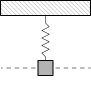
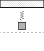
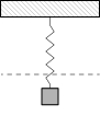
We convert between mass and weight using the formula¹⁷ $w = m g$ . Here, $w$ is the weight of the object, $m$ is the mass and $g$ is the acceleration due to gravity. In the English system, $g = 32 \frac{feet}{{second}^{2}}$ , and in the SI system, $g = 9.8 \frac{meters}{{second}^{2}}$ . Hence, on Earth a mass of 1 slug weighs 32 lbs. and a mass of 1 kg weighs 9.8 N.¹⁸ Suppose we attach an object with mass $m$ to a spring as depicted below.

t]ccc

Coordinate-plane figure. — **Figure 12.87**

$x ⁢ open parenthesis t close parenthesis equals 0$ at the

$x ⁢ open parenthesis t close parenthesis less than 0$ above the

$x ⁢ open parenthesis t close parenthesis greater than 0$ below the

equilibrium position

The weight of the object will stretch the spring. The system is said to be in `equilibrium' when the weight of the object is perfectly balanced with the restorative force of the spring. How far the spring stretches to reach equilibrium depends on the spring's `spring constant'. Usually denoted by the letter $k$ , the spring constant relates the force $F$ applied to the spring to the amount $d$ the spring stretches in accordance with Hooke's Law ¹⁹ $F = k d$ .

If the object is released above or below the equilibrium position, or if the object is released with an upward or downward velocity, the object will bounce up and down on the end of the spring until some external force stops it. If we let $x (t)$ denote the object's displacement from the equilibrium position at time $t$ , then $x ⁢ open parenthesis t close parenthesis equals 0$ means the object is at the equilibrium position, $x ⁢ open parenthesis t close parenthesis less than 0$ means the object is above the equilibrium position, and $x ⁢ open parenthesis t close parenthesis greater than 0$ means the object is below the equilibrium position. The function $x (t)$ is called the `equation of motion' of the object.²⁰

If we ignore all other influences on the system except gravity and the spring force, then Physics tells us that gravity and the spring force will battle each other forever and the object will oscillate indefinitely. In this case, we describe the motion as `free' (meaning there is no external force causing the motion) and `undamped' (meaning we ignore friction caused by surrounding medium, which in our case is air).

The following theorem, which comes from Differential Equations, gives $x (t)$ as a function of the mass $m$ of the object, the spring constant $k$ , the initial displacement $x sub 0$ of the object and initial velocity $v sub 0$ of the object.

As with $x (t)$ , $x sub 0 equals 0$ means the object is released from the equilibrium position, $x sub 0 less than 0$ means the object is released above the equilibrium position and $x sub 0 greater than 0$ means the object is released below the equilibrium position. As far as the initial velocity $v sub 0$ is concerned, $v sub 0 equals 0$ means the object is released `from rest,' $v sub 0 less than 0$ means the object is heading upwards and $v sub 0 greater than 0$ means the object is heading downwards.²¹

Theorem

Equation for Free Undamped Harmonic Motion: Suppose an object of mass $m$ is suspended from a spring with spring constant $k$ . If the initial displacement from the equilibrium position is $x sub 0$ and the initial velocity of the object is $v sub 0$ , then the displacement $x$ from the equilibrium position at time $t$ is given by $x (t) = A \sin (ω t + ϕ)$ where

$ω = \sqrt{\frac{k}{m}}$ and $A = \sqrt{x_{0}^{2} + {(\frac{v_{0}}{ω})}^{2}}$
$A ⁢ sin ⁡ open parenthesis ϕ close parenthesis equals x sub 0$ and $A ⁢ ω ⁢ cos ⁡ open parenthesis ϕ close parenthesis equals v sub 0$ .

It is a great exercise in `dimensional analysis' to verify that the formulas given in Theorem 12.18 work out so that $ω$ has units $\frac{1}{s}$ and $A$ has units ft. or m, depending on which system we choose.

Example 6

Suppose an object weighing 64 pounds stretches a spring 8 feet.

If the object is attached to the spring and released 3 feet below the equilibrium position from rest, find the equation of motion of the object, $x (t)$ . When does the object first pass through the equilibrium position? Is the object heading upwards or downwards at this instant?
If the object is attached to the spring and released 3 feet below the equilibrium position with an upward velocity of $8$ feet per second, find the equation of motion of the object, $x (t)$ . What is the longest distance the object travels above the equilibrium position? When does this first happen? Confirm your result using a graphing utility.

In order to use the formulas in Theorem 12.18, we first need to determine the spring constant $k$ and the mass of the object $m$ .

To find $k$ , we use Hooke's Law $F = k d$ . We know the object weighs $64$ lbs. and stretches the spring $8$ ft.. Using $F equals 64$ and $d equals 8$ , we get $64 = k \cdot 8$ , or $k = 8 \frac{lbs.}{ft.}$ .

To find $m$ , we use $w = m g$ with $w equals 64$ lbs. and $g = 32 \frac{ft.}{s^{2}}$ . We get $m equals 2$ slugs. We can now proceed to apply Theorem 12.18.

With $k equals 8$ and $m equals 2$ , we get $ω = \sqrt{\frac{k}{m}} = \sqrt{\frac{8}{2}} = 2$ . Since the object is released 3 feet below the equilibrium position `from rest,' $x sub 0 equals 3$ and $v sub 0 equals 0$ . Therefore, $A = \sqrt{x_{0}^{2} + {(\frac{v_{0}}{ω})}^{2}} = \sqrt{3^{2} + 0^{2}} = 3$ .
To determine the phase $ϕ$ , we have $A ⁢ sin ⁡ open parenthesis ϕ close parenthesis equals x sub 0$ , which in this case gives $3 ⁢ sin ⁡ open parenthesis ϕ close parenthesis equals 3$ so $sin ⁡ open parenthesis ϕ close parenthesis equals 1$ . Only $ϕ = \frac{π}{2}$ and angles coterminal to it satisfy this condition, so we pick²² the phase to be $ϕ = \frac{π}{2}$ . Hence, the equation of motion is $x (t) = 3 \sin (2 t + \frac{π}{2})$ .
To find when the object passes through the equilibrium position we solve $x (t) = 3 \sin (2 t + \frac{π}{2}) = 0$ . Going through the usual analysis we find $t = - \frac{π}{4} + \frac{π}{2} k$ for integers $k$ . Since we are interested in the first time the object passes through the equilibrium position, we look for the smallest positive $t$ value which in this case is $t = \frac{π}{4} \approx 0.78$ seconds after the start of the motion.
Common sense suggests that if we release the object below the equilibrium position, the object should be traveling upwards when it first passes through it. To check this answer, we graph one cycle of $x (t)$ . Since our applied domain in this situation is $t greater than or equal to 0$ , and the period of $x (t)$ is $T = \frac{2 π}{ω} = \frac{2 π}{2} = π$ , we graph $x (t)$ over the interval $open bracket 0, π close bracket$ . Remembering that $x ⁢ open parenthesis t close parenthesis greater than 0$ means the object is below the equilibrium position and $x ⁢ open parenthesis t close parenthesis less than 0$ means the object is above the equilibrium position, the fact our graph is crossing through the $t$ -axis from positive $x$ to negative $x$ at $t = \frac{π}{4}$ confirms our answer.
Figure 12.90
$x (t) = 3 \sin (2 t + \frac{π}{2})$
The only difference between this problem and the previous problem is that we now release the object with an upward velocity of $8 \frac{ft}{s}$ . We still have $ω equals 2$ and $x sub 0 equals 3$ , but now we have $v_{0} = - 8$ , the negative indicating the velocity is directed upwards.
Here, we get $A = \sqrt{x_{0}^{2} + {(\frac{v_{0}}{ω})}^{2}} = \sqrt{3^{2} + {(- 4)}^{2}} = 5$ . From $A ⁢ sin ⁡ open parenthesis ϕ close parenthesis equals x sub 0$ , we get $5 ⁢ sin ⁡ open parenthesis ϕ close parenthesis equals 3$ which gives $\sin (ϕ) = \frac{3}{5}$ . From $A ⁢ ω ⁢ cos ⁡ open parenthesis ϕ close parenthesis equals v sub 0$ , we get $10 \cos (ϕ) = - 8$ , or $\cos (ϕ) = - \frac{4}{5}$ .
Hence, $ϕ$ is a Quadrant II angle which we can describe in terms of either arcsine or arccosine. Since the range of arccosine covers Quadrant II, we choose to express $ϕ$ in terms of the arccosine: $ϕ = \arccos (- \frac{4}{5})$ . Hence, $x (t) = 5 \sin (2 t + \arccos (- \frac{4}{5}))$ .
Since the amplitude of $x (t)$ is $5$ , the object will travel at most $5$ feet above the equilibrium position. To find when this happens, we solve the equation $x (t) = 5 \sin (2 t + \arccos (- \frac{4}{5})) = - 5$ , the negative once again signifying that the object is above the equilibrium position.
Going through the usual machinations, we get $t = - \frac{1}{2} \arccos (- \frac{4}{5}) - \frac{π}{4} + π k$ for integers $k$ . The smallest (positive) of these values occurs when $k equals 1$ , that is, $t = - \frac{1}{2} \arccos (- \frac{4}{5}) + \frac{3 π}{4} \approx 1.107$ seconds after the start of the motion.
Graphing $x (t) = 5 \sin (2 t + \arccos (- \frac{4}{5}))$ , we find the coordinates of the first relative minimum of to be approximately $open parenthesis 1.107, minus 5 close parenthesis$ .
Figure 12.91
$x (t) = 5 \sin (2 t + \arccos (- \frac{4}{5}))$

Though beyond the scope of this course, it is possible to model the effects of friction and other external forces acting on the system.²³

While we may not have the Physics and Calculus background to derive equations of motion for these scenarios, we can certainly analyze them. We examine three cases in the following example.

Example 7

Write $x (t) = 5 e^{- t / 5} \cos (t) + 5 e^{- t / 5} \sqrt{3} \sin (t)$ in the form $x (t) = A (t) \sin (ω t + ϕ)$ . Graph $x (t)$ using a graphing utility.
Write $x (t) = (t + 3) \sqrt{2} \cos (2 t) + (t + 3) \sqrt{2} \sin (2 t)$ in the form $x (t) = A (t) \sin (ω t + ϕ)$ . Graph $x (t)$ using a graphing utility.
Find the period of $x (t) = 5 \sin (6 t) - 5 \sin (8 t)$ . Graph $x (t)$ using a graphing utility.

We start rewriting $x (t) = 5 e^{- t / 5} \cos (t) + 5 e^{- t / 5} \sqrt{3} \sin (t)$ by factoring out $5 e^{- t / 5}$ from both terms to get $x (t) = 5 e^{- t / 5} (\cos (t) + \sqrt{3} \sin (t))$ . We convert what's left in parentheses to the required form using the technique introduced in Example 12.2.1 from Section 12.2. We find $(\cos (t) + \sqrt{3} \sin (t)) = 2 \sin (t + \frac{π}{3})$ so that $x (t) = 10 e^{- t / 5} \sin (t + \frac{π}{3})$ .
Graphing $x (t)$ reveals some interesting behavior. The sinusoidal nature continues indefinitely, but it is being attenuated. In the sinusoid $A \sin (ω t + ϕ)$ , the coefficient $A$ of the sine function is the amplitude. In the case of $x (t) = 10 e^{- t / 5} \sin (t + \frac{π}{3})$ , we can think of the function $A (t) = 10 e^{- t / 5}$ as the amplitude.²⁴ Since $lim_{t \to \infty} 10 e^{- t / 5} = 0$ , we can use the Squeeze Theorem, Theorem 10.2 that $lim t → ∞ x ⁢ open parenthesis t close parenthesis equals 0$ . (See Exercise ).
Indeed, if we graph $x = \pm 10 e^{- t / 5}$ along with $x (t) = 10 e^{- t / 5} \sin (t + \frac{π}{3})$ , we see this attenuation taking place with the exponentials acting as a `wave envelope.'
Figure 12.92
$x (t) = 10 e^{- t / 5} \sin (t + \frac{π}{3})$ and $x = \pm 10 e^{- t / 5}$
In this case, the function $x (t)$ corresponds to the motion of an object on a spring where there is a slight force which acts to `damp', or slow the motion. An example of this kind of force would be the friction of the object against the air. According to this model, the object oscillates forever, but with increasingly smaller and smaller amplitude. This motion is often described as underdamped motion.
Proceeding as in the first example, we factor out $(t + 3) \sqrt{2}$ from each term in the function $x (t)$ to get $x (t) = (t + 3) \sqrt{2} (\cos (2 t) + \sin (2 t))$ . We find $(\cos (2 t) + \sin (2 t)) = \sqrt{2} \sin (2 t + \frac{π}{4})$ , so an equivalent form of $x (t)$ is $x (t) = 2 (t + 3) \sin (2 t + \frac{π}{4})$ .
Graphing $x (t)$ , we find the sinusoid's amplitude growing. This isn't too surprising since our amplitude function here is $A (t) = 2 (t + 3) = 2 t + 6$ , grows without bound as $t → ∞$ .
Figure 12.93
$x (t) = 2 (t + 3) \sin (2 t + \frac{π}{4})$ and $x = \pm 2 (t + 3)$
The phenomenon illustrated here is `forced' motion. That is, we imagine that the entire apparatus on which the spring is attached is oscillating as well.
In this particular case, we are witnessing a `resonance' effect – the frequency of the external oscillation matches the frequency of the motion of the object on the spring. In a mechanical system, this will result in some sort of structural failure.²⁵
Last, but not least, we come to $x (t) = 5 \sin (6 t) - 5 \sin (8 t)$ . To find the period of this function, we need to determine the length of the smallest interval on which both $f ⁢ open parenthesis t close parenthesis equals 5 ⁢ sin ⁡ open parenthesis 6 ⁢ t close parenthesis$ and $g ⁢ open parenthesis t close parenthesis equals 5 ⁢ sin ⁡ open parenthesis 8 ⁢ t close parenthesis$ complete a whole number of cycles.
To do this, we take the ratio of their frequencies and reduce to lowest terms: $\frac{6}{8} = \frac{3}{4}$ . This tells us that for every $3$ cycles $f$ makes, $g$ makes $4$ . Hence, the period of $x (t)$ is three times the period of $f (t)$ (which is four times the period of $g (t)$ ), or $π$ . We check our work by graphing $x (t)$ over $open bracket 0, π close bracket$
The reader may recognize $x (t)$ an example of the `beats' phenomenon we first saw on in Section 12.2.1. Indeed, using a sum to product identity, we may rewrite $x (t)$ as $x (t) = - 10 \sin (t) \cos (7 t)$ . As we saw on (and Exercises - in Section 12.2), the lower frequency factor, $minus 10 ⁢ sin ⁡ open parenthesis t close parenthesis$ determines the `wave-envelope,' $x = \pm 10 \sin (t)$ .
Figure 12.94
$x (t) = 5 \sin (6 t) - 5 \sin (8 t)$ and $x = \pm 10 \sin (t)$ over $open bracket 0, π close bracket$
This equation of motion also results from `forced' motion, but here the frequency of the external oscillation is different than that of the object on the spring. Since the sinusoids here have different frequencies, they are `out of sync' and do not amplify each other as in the previous example. Instead, through a combination of constructive and destructive interference, the mass continues to oscillate no more than $10$ units from its equilibrium position indefinitely.

Our last examples use the tools of this section along with those developed in Section 6.3.

Example 8

Let $f (x) = 2 \sin (x) - \sin (2 x)$ restricted to the interval $open bracket 0, 2 ⁢ π close bracket$ .

Given $f^{'} (x) = 2 \cos (x) - 2 \cos (2 x)$ , find the open intervals over which $f$ is increasing and decreasing.
Locate all relative extrema and check your answers graphically.

We begin making a sign diagram for $f^{'} (x) = 2 \cos (x) - 2 \cos (2 x)$ by solving $f prime ⁢ open parenthesis x close parenthesis equals 0$ :

Table 12.1

f^{'} (x)

=

0

2 ⁢ cos ⁡ open parenthesis x close parenthesis minus 2 ⁢ cos ⁡ open parenthesis 2 ⁢ x close parenthesis

=

0

2 \cos (x) - 2 (2 \cos^{2} (x) - 1)

=

0

Double Angle Identity:

\cos (2 x) = 2 \cos^{2} (x) - 1

2 \cos (x) - 4 \cos^{2} (x) + 2

=

0

- 2 (2 \cos^{2} (x) - \cos (x) - 1)

=

0

- 2 (2 \cos (x) + 1) (\cos (x) - 1)

=

0

We get $2 \cos (x) + 1 = 0$ or $\cos (x) = - \frac{1}{2}$ . In the interval $open parenthesis 0, 2 ⁢ π close parenthesis$ , the only solutions are $x = \frac{2 π}{3}$ and $x = \frac{4 π}{3}$ . We also get $\cos (x) - 1 = 0$ or $cos ⁡ open parenthesis x close parenthesis equals 1$ which occurs at the endpoints $x equals 0$ and $x equals 2 ⁢ π$ .

We create our sign diagram for $f^{'} (x)$ and interpret what it means for $f (x)$ below.

Figure 12.95

Figure 12.96

We find $f$ is increasing on $(0, \frac{2 π}{3})$ and $(\frac{4 π}{3}, 2 π)$ and $f$ is decreasing on $(\frac{2 π}{3}, \frac{4 π}{3})$ .

Using the sign diagram along with the First Derivative Test, Theorem 6.5, we find that $f$ has a local maximum: $(\frac{2 π}{3}, f (\frac{2 π}{3})) = (\frac{2 π}{3}, \frac{3 \sqrt{3}}{2})$ and a local minimum: $(\frac{4 π}{3}, f (\frac{4 π}{3})) = (\frac{4 π}{3}, - \frac{3 \sqrt{3}}{2})$ . Both of these extrema are absolute (global) as well as local.
Figure 12.97

We'll continue our work with $f (x) = 2 \sin (x) - \sin (2 x)$ from Example 12.4.8 in Exercise.

Example 9

Let $f (x) = x - 2 \cos (x)$ restricted to the interval $0 less than or equal to x less than or equal to 2 ⁢ π$ .

Given $f double prime ⁢ open parenthesis x close parenthesis equals 2 ⁢ cos ⁡ open parenthesis x close parenthesis$ , find the inflection points of the graph. Check your answer graphically.

We make a sign digram for $f^{''} (x)$ , first solving $f^{''} (x) = 2 \cos (x) = 0$ . We get $x = \frac{π}{2}$ and $x = \frac{3 π}{2}$ .

Figure 12.98

Figure 12.99

We see the concavity changes at both $x = \frac{π}{2}$ and $x = \frac{3 π}{2}$ so we have inflection points: $(\frac{π}{2}, f (\frac{π}{2})) = (\frac{π}{2}, \frac{π}{2})$ and $(\frac{3 π}{2}, f (\frac{3 π}{2})) = (\frac{3 π}{2}, \frac{3 π}{2})$ .

Figure 12.100

We'll revisit $f (x) = x - 2 \cos (x)$ from Example 12.4.9 in Exercise. Speaking of Exercises …

Exercises

In Exercises -, find all of the exact solutions of the equation and then list those solutions which are in the interval $open bracket 0, 2 ⁢ π close parenthesis$ .

$sin ⁡ open parenthesis 5 ⁢ θ close parenthesis equals 0$
$\cos (3 t) = \frac{1}{2}$
$\sin (- 2 x) = \frac{\sqrt{3}}{2}$
$tan ⁡ open parenthesis 6 ⁢ θ close parenthesis equals 1$
$\csc (4 t) = - 1$
$\sec (3 x) = \sqrt{2}$
$\cot (2 θ) = - \frac{\sqrt{3}}{3}$
$cos ⁡ open parenthesis 9 ⁢ t close parenthesis equals 9$
$\sin (\frac{x}{3}) = \frac{\sqrt{2}}{2}$
$\cos (θ + \frac{5 π}{6}) = 0$
$\sin (2 t - \frac{π}{3}) = - \frac{1}{2}$
$2 \cos (x + \frac{7 π}{4}) = \sqrt{3}$
$csc ⁡ open parenthesis θ close parenthesis equals 0$
$\tan (2 t - π) = 1$
$tan squared ⁡ open parenthesis x close parenthesis equals 3$
$\sec^{2} (θ) = \frac{4}{3}$
$\cos^{2} (t) = \frac{1}{2}$
$\sin^{2} (x) = \frac{3}{4}$

In Exercises -, solve the equation, giving the exact solutions which lie in $open bracket 0, 2 ⁢ π close parenthesis$

$\sin (θ) = \cos (θ)$
$sin ⁡ open parenthesis 2 ⁢ t close parenthesis equals sin ⁡ open parenthesis t close parenthesis$
$sin ⁡ open parenthesis 2 ⁢ x close parenthesis equals cos ⁡ open parenthesis x close parenthesis$
$cos ⁡ open parenthesis 2 ⁢ θ close parenthesis equals sin ⁡ open parenthesis θ close parenthesis$
$cos ⁡ open parenthesis 2 ⁢ t close parenthesis equals cos ⁡ open parenthesis t close parenthesis$
$\cos (2 x) = 2 - 5 \cos (x)$
$3 \cos (2 θ) + \cos (θ) + 2 = 0$
$\cos (2 t) = 5 \sin (t) - 2$
$3 \cos (2 x) = \sin (x) + 2$
$2 \sec^{2} (θ) = 3 - \tan (θ)$
$\tan^{2} (t) = 1 - \sec (t)$
$\cot^{2} (x) = 3 \csc (x) - 3$
$sec ⁡ open parenthesis θ close parenthesis equals 2 ⁢ csc ⁡ open parenthesis θ close parenthesis$
$\cos (t) \csc (t) \cot (t) = 6 - \cot^{2} (t)$
$sin ⁡ open parenthesis 2 ⁢ x close parenthesis equals tan ⁡ open parenthesis x close parenthesis$
$\cot^{4} (θ) = 4 \csc^{2} (θ) - 7$
$\cos (2 t) + \csc^{2} (t) = 0$
$tan cubed ⁡ open parenthesis x close parenthesis equals 3 ⁢ tan ⁡ open parenthesis x close parenthesis$
$\tan^{2} (θ) = \frac{3}{2} \sec (θ)$
$\cos^{3} (t) = - \cos (t)$
$\tan (2 x) - 2 \cos (x) = 0$
$\csc^{3} (θ) + \csc^{2} (θ) = 4 \csc (θ) + 4$
$2 \tan (t) = 1 - \tan^{2} (t)$
$\tan (x) = \sec (x)$

In Exercises -, solve the equation, giving the exact solutions which lie in $open bracket 0, 2 ⁢ π close parenthesis$

$\sin (6 θ) \cos (θ) = - \cos (6 θ) \sin (θ)$
$sin ⁡ open parenthesis 3 ⁢ t close parenthesis ⁢ cos ⁡ open parenthesis t close parenthesis equals cos ⁡ open parenthesis 3 ⁢ t close parenthesis ⁢ sin ⁡ open parenthesis t close parenthesis$
$\cos (2 x) \cos (x) + \sin (2 x) \sin (x) = 1$
$\cos (5 θ) \cos (3 θ) - \sin (5 θ) \sin (3 θ) = \frac{\sqrt{3}}{2}$
$\sin (t) + \cos (t) = 1$
$\sin (x) + \sqrt{3} \cos (x) = 1$
$\sqrt{2} \cos (θ) - \sqrt{2} \sin (θ) = 1$
$\sqrt{3} \sin (2 t) + \cos (2 t) = 1$
$\cos (2 x) - \sqrt{3} \sin (2 x) = \sqrt{2}$
$3 \sqrt{3} \sin (3 θ) - 3 \cos (3 θ) = 3 \sqrt{3}$
$cos ⁡ open parenthesis 3 ⁢ t close parenthesis equals cos ⁡ open parenthesis 5 ⁢ t close parenthesis$
$cos ⁡ open parenthesis 4 ⁢ x close parenthesis equals cos ⁡ open parenthesis 2 ⁢ x close parenthesis$
$sin ⁡ open parenthesis 5 ⁢ θ close parenthesis equals sin ⁡ open parenthesis 3 ⁢ θ close parenthesis$
$\cos (5 t) = - \cos (2 t)$
$\sin (6 x) + \sin (x) = 0$
$\tan (x) = \cos (x)$

In Exercises -, solve the equation.

$arccos ⁡ open parenthesis 2 ⁢ x close parenthesis equals π$
$π - 2 \arcsin (t) = 2 π$
$4 \arctan (3 x - 1) - π = 0$
$6 arccot (2 t) - 5 π = 0$
$4 arcsec (\frac{x}{2}) = π$
$12 arccsc (\frac{t}{3}) = 2 π$
$9 \arcsin^{2} (x) - π^{2} = 0$
$9 \arccos^{2} (t) - π^{2} = 0$
$8 {arccot}^{2} (x) + 3 π^{2} = 10 π arccot (x)$
$6 \arctan {(t)}^{2} = π \arctan (x) + π^{2}$

In Exercises -, solve the inequality. Express the exact answer in interval notation, restricting your attention to $0 less than or equal to x less than or equal to 2 ⁢ π$ .

$sin ⁡ open parenthesis x close parenthesis less than or equal to 0$
$tan ⁡ open parenthesis t close parenthesis greater than or equal to the square root of 3$
$sec squared ⁡ open parenthesis x close parenthesis less than or equal to 4$
$\cos^{2} (t) > \frac{1}{2}$
$cos ⁡ open parenthesis 2 ⁢ x close parenthesis less than or equal to 0$
$\sin (t + \frac{π}{3}) > \frac{1}{2}$
$\cot^{2} (x) \geq \frac{1}{3}$
$2 ⁢ cos ⁡ open parenthesis t close parenthesis greater than or equal to 1$
$sin ⁡ open parenthesis 5 ⁢ x close parenthesis greater than or equal to 5$
$cos ⁡ open parenthesis 3 ⁢ t close parenthesis less than or equal to 1$
$sec ⁡ open parenthesis x close parenthesis less than or equal to the square root of 2$
$cot ⁡ open parenthesis t close parenthesis less than or equal to 4$

In Exercises -, solve the inequality. Express the exact answer in interval notation, restricting your attention to $- π \leq x \leq π$ .

$\cos (x) > \frac{\sqrt{3}}{2}$
$\sin (t) > \frac{1}{3}$
$sec ⁡ open parenthesis x close parenthesis less than or equal to 2$
$\sin^{2} (t) < \frac{3}{4}$
$cot ⁡ open parenthesis x close parenthesis greater than or equal to minus 1$
$\cos (t) \geq \sin (t)$

In Exercises -, solve the inequality. Express the exact answer in interval notation, restricting your attention to $minus 2 ⁢ π less than or equal to x less than or equal to 2 ⁢ π$ .

$csc ⁡ open parenthesis x close parenthesis greater than 1$
$\cos (t) \leq \frac{5}{3}$
$cot ⁡ open parenthesis x close parenthesis greater than or equal to 5$
$tan squared ⁡ open parenthesis t close parenthesis greater than or equal to 1$
$sin ⁡ open parenthesis 2 ⁢ x close parenthesis greater than or equal to sin ⁡ open parenthesis x close parenthesis$
$cos ⁡ open parenthesis 2 ⁢ t close parenthesis less than or equal to sin ⁡ open parenthesis x close parenthesis$

In Exercises -, solve the given inequality.

$arcsin ⁡ open parenthesis 2 ⁢ x close parenthesis greater than 0$
$3 ⁢ arccos ⁡ open parenthesis t close parenthesis less than or equal to π$
$6 ⁢ arccot ⁢ open parenthesis 7 ⁢ x close parenthesis greater than or equal to π$
$π greater than 2 ⁢ arctan ⁡ open parenthesis t close parenthesis$
$2 arcsin open parenthesis x close parenthesis squared greater than π arcsin open parenthesis x close parenthesis$
$12 arccos open parenthesis t close parenthesis squared plus 2 π squared greater than 11 π arccos open parenthesis t close parenthesis$

In Exercises -, express the domain of the function using the extended interval notation. (See Example 12.4.4 and Section 11.5.3 for details.)

$f (x) = \frac{1}{\cos (x) - 1}$
$f (t) = \frac{\cos (t)}{\sin (t) + 1}$
$f (x) = \sqrt{\tan^{2} (x) - 1}$
$f (t) = \sqrt{2 - \sec (t)}$
$f ⁢ open parenthesis x close parenthesis equals csc ⁡ open parenthesis 2 ⁢ x close parenthesis$
$f (t) = \frac{\sin (t)}{2 + \cos (t)}$
$f (x) = 3 \csc (x) + 4 \sec (x)$
$f (t) = \ln (| \cos (t) |)$
$f (x) = \arcsin (\tan (x))$
1. With the help of your classmates, determine the number of solutions to $\sin (x) = \frac{1}{2}$ in $open bracket 0, 2 ⁢ π close parenthesis$ . Then find the number of solutions to $\sin (2 x) = \frac{1}{2}$ , $\sin (3 x) = \frac{1}{2}$ and $\sin (4 x) = \frac{1}{2}$ in $open bracket 0, 2 ⁢ π close parenthesis$ . What pattern emerges? Explain how this pattern would help you solve equations like $\sin (11 x) = \frac{1}{2}$ .
2. Repeat the above exercise focusing on $\sin (\frac{x}{2}) = \frac{1}{2}$ , $\sin (\frac{3 x}{2}) = \frac{1}{2}$ and $\sin (\frac{5 x}{2}) = \frac{1}{2}$ . What pattern emerges here?
3. Replace sine with tangent and $\frac{1}{2}$ with $1$ and repeat the whole exploration.
Suppose an object weighing $10$ pounds is suspended from the ceiling by a spring which stretches $2$ feet to its equilibrium position when the object is attached.
1. Find the spring constant $k$ in $\frac{lbs.}{ft.}$ and the mass of the object in slugs.
2. Find the equation of motion of the object if it is released from $1$ foot below the equilibrium position from rest. When is the first time the object passes through the equilibrium position? In which direction is it heading?
3. Find the equation of motion of the object if it is released from $6$ inches above the equilibrium position with a downward velocity of $2$ feet per second. Find when the object passes through the equilibrium position heading downwards for the third time.
In Example 12.4.8, $f (x) = 2 \sin (x) - \sin (2 x)$ restricted to $0 less than or equal to x less than or equal to 2 ⁢ π$ . If $f^{''} (x) = 4 \sin (2 x) - 2 \sin (x)$ , find the inflection points of the graph of $y = f (x)$ .
In Example 12.4.9, $f (x) = x - 2 \cos (x)$ restricted to $0 less than or equal to x less than or equal to 2 ⁢ π$ . If $f^{'} (x) = 2 \sin (x) + 1$ , list the open intervals over which $f$ is increasing and decreasing. Find the local extrema.
Let $f (x) = e^{- x} \sin (x)$ for $x greater than 0$ .
1. Use the Squeeze Theorem, Theorem 10.2, to find $lim x → ∞ f ⁢ open parenthesis x close parenthesis$ . Interpret your answer graphically.
  HINT: Since $minus 1 less than or equal to sin ⁡ open parenthesis x close parenthesis less than or equal to 1$ , $- e^{- x} \leq e^{- x} \sin (x) \leq e^{- x}$ …
2. Use the fact that $f^{'} (x) = e^{- x} \cos (x) - e^{- x} \sin (x)$ to help you find the intervals over which $f$ is increasing and decreasing.
3. Use the fact that $f^{''} (x) = - 2 e^{- x} \cos (x)$ to help you find the intervals over which the graph of $f$ is concave up and concave down.
Recall $x (t) = 10 e^{- t / 5} \sin (t + \frac{π}{3})$ from Example 12.4.7 number models underdamped motion. Use the Squeeze Theorem, Theorem 10.2, to prove $lim t → ∞ x ⁢ open parenthesis t close parenthesis equals 0$ .
HINT: Since $- 1 \leq \sin (t + \frac{π}{3}) \leq 1$ , $- 10 e^{- t / 5} \leq 10 e^{- t / 5} \sin (t + \frac{π}{3}) \leq 10 e^{- t / 5}$ …

Answers

$θ = \frac{π k}{5}; θ = 0, \frac{π}{5}, \frac{2 π}{5}, \frac{3 π}{5}, \frac{4 π}{5}, π, \frac{6 π}{5}, \frac{7 π}{5}, \frac{8 π}{5}, \frac{9 π}{5}$
$t = \frac{π}{9} + \frac{2 π k}{3}$ or $t = \frac{5 π}{9} + \frac{2 π k}{3}; t = \frac{π}{9}, \frac{5 π}{9}, \frac{7 π}{9}, \frac{11 π}{9}, \frac{13 π}{9}, \frac{17 π}{9}$
$x = \frac{2 π}{3} + π k$ or $x = \frac{5 π}{6} + π k; x = \frac{2 π}{3}, \frac{5 π}{6}, \frac{5 π}{3}, \frac{11 π}{6}$
$θ = \frac{π}{24} + \frac{π k}{6}; θ = \frac{π}{24}, \frac{5 π}{24}, \frac{3 π}{8}, \frac{13 π}{24}, \frac{17 π}{24}, \frac{7 π}{8}, \frac{25 π}{24}, \frac{29 π}{24}, \frac{11 π}{8}, \frac{37 π}{24}, \frac{41 π}{24}, \frac{15 π}{8}$
$t = \frac{3 π}{8} + \frac{π k}{2}; t = \frac{3 π}{8}, \frac{7 π}{8}, \frac{11 π}{8}, \frac{15 π}{8}$
$x = \frac{π}{12} + \frac{2 π k}{3}$ or $x = \frac{7 π}{12} + \frac{2 π k}{3}; x = \frac{π}{12}, \frac{7 π}{12}, \frac{3 π}{4}, \frac{5 π}{4}, \frac{17 π}{12}, \frac{23 π}{12}$
$θ = \frac{π}{3} + \frac{π k}{2}; θ = \frac{π}{3}, \frac{5 π}{6}, \frac{4 π}{3}, \frac{11 π}{6}$
No solution
$x = \frac{3 π}{4} + 6 π k$ or $x = \frac{9 π}{4} + 6 π k; x = \frac{3 π}{4}$
$θ = - \frac{π}{3} + π k; θ = \frac{2 π}{3}, \frac{5 π}{3}$
$t = \frac{3 π}{4} + π k$ or $t = \frac{13 π}{12} + π k; t = \frac{π}{12}, \frac{3 π}{4}, \frac{13 π}{12}, \frac{7 π}{4}$
$x = - \frac{19 π}{12} + 2 π k$ or $x = \frac{π}{12} + 2 π k; x = \frac{π}{12}, \frac{5 π}{12}$
No solution
$t = \frac{5 π}{8} + \frac{π k}{2}; t = \frac{π}{8}, \frac{5 π}{8}, \frac{9 π}{8}, \frac{13 π}{8}$
$x = \frac{π}{3} + π k$ or $x = \frac{2 π}{3} + π k; x = \frac{π}{3}, \frac{2 π}{3}, \frac{4 π}{3}, \frac{5 π}{3}$
$θ = \frac{π}{6} + π k$ or $θ = \frac{5 π}{6} + π k; θ = \frac{π}{6}, \frac{5 π}{6}, \frac{7 π}{6}, \frac{11 π}{6}$
$t = \frac{π}{4} + \frac{π k}{2}; t = \frac{π}{4}, \frac{3 π}{4}, \frac{5 π}{4}, \frac{7 π}{4}$
$x = \frac{π}{3} + π k$ or $x = \frac{2 π}{3} + π k; x = \frac{π}{3}, \frac{2 π}{3}, \frac{4 π}{3}, \frac{5 π}{3}$
$θ = \frac{π}{4}, \frac{5 π}{4}$
$t = 0, \frac{π}{3}, π, \frac{5 π}{3}$
$x = \frac{π}{6}, \frac{π}{2}, \frac{5 π}{6}, \frac{3 π}{2}$
$θ = \frac{π}{6}, \frac{5 π}{6}, \frac{3 π}{2}$
$t = 0, \frac{2 π}{3}, \frac{4 π}{3}$
$x = \frac{π}{3}, \frac{5 π}{3}$
$θ = \frac{2 π}{3}, \frac{4 π}{3}, \arccos (\frac{1}{3}), 2 π - \arccos (\frac{1}{3})$
$t = \frac{π}{6}, \frac{5 π}{6}$
$x = \frac{7 π}{6}, \frac{11 π}{6}, \arcsin (\frac{1}{3}), π - \arcsin (\frac{1}{3})$
$θ = \frac{3 π}{4}, \frac{7 π}{4}, \arctan (\frac{1}{2}), π + \arctan (\frac{1}{2})$
$t = 0, \frac{2 π}{3}, \frac{4 π}{3}$
$x = \frac{π}{6}, \frac{5 π}{6}, \frac{π}{2}$
$θ = \arctan (2), π + \arctan (2)$
$t = \frac{π}{6}, \frac{7 π}{6}, \frac{5 π}{6}, \frac{11 π}{6}$
$x = 0, π, \frac{π}{4}, \frac{3 π}{4}, \frac{5 π}{4}, \frac{7 π}{4}$
$θ = \frac{π}{6}, \frac{π}{4}, \frac{3 π}{4}, \frac{5 π}{6}, \frac{7 π}{6}, \frac{5 π}{4}, \frac{7 π}{4}, \frac{11 π}{6}$
$t = \frac{π}{2}, \frac{3 π}{2}$
$x = 0, \frac{π}{3}, \frac{2 π}{3}, π, \frac{4 π}{3}, \frac{5 π}{3}$
$θ = \frac{π}{3}, \frac{5 π}{3}$
$t = \frac{π}{2}, \frac{3 π}{2}$
$x = \frac{π}{6}, \frac{π}{2}, \frac{5 π}{6}, \frac{3 π}{2}$
$θ = \frac{π}{6}, \frac{5 π}{6}, \frac{7 π}{6}, \frac{3 π}{2}, \frac{11 π}{6}$
$t = \frac{π}{8}, \frac{5 π}{8}, \frac{9 π}{8}, \frac{13 π}{8}$
No solution
$θ = 0, \frac{π}{7}, \frac{2 π}{7}, \frac{3 π}{7}, \frac{4 π}{7}, \frac{5 π}{7}, \frac{6 π}{7}, π, \frac{8 π}{7}, \frac{9 π}{7}, \frac{10 π}{7}, \frac{11 π}{7}, \frac{12 π}{7}, \frac{13 π}{7}$
$t = 0, \frac{π}{2}, π, \frac{3 π}{2}$
$x equals 0$
$θ = \frac{π}{48}, \frac{11 π}{48}, \frac{13 π}{48}, \frac{23 π}{48}, \frac{25 π}{48}, \frac{35 π}{48}, \frac{37 π}{48}, \frac{47 π}{48}, \frac{49 π}{48}, \frac{59 π}{48}, \frac{61 π}{48}, \frac{71 π}{48}, \frac{73 π}{48}, \frac{83 π}{48}, \frac{85 π}{48}, \frac{95 π}{48}$
$t = 0, \frac{π}{2}$
$x = \frac{π}{2}, \frac{11 π}{6}$
$θ = \frac{π}{12}, \frac{17 π}{12}$
$t = 0, π, \frac{π}{3}, \frac{4 π}{3}$
$x = \frac{17 π}{24}, \frac{41 π}{24}, \frac{23 π}{24}, \frac{47 π}{24}$
$θ = \frac{π}{6}, \frac{5 π}{18}, \frac{5 π}{6}, \frac{17 π}{18}, \frac{3 π}{2}, \frac{29 π}{18}$
$t = 0, \frac{π}{4}, \frac{π}{2}, \frac{3 π}{4}, π, \frac{5 π}{4}, \frac{3 π}{2}, \frac{7 π}{4}$
$x = 0, \frac{π}{3}, \frac{2 π}{3}, π, \frac{4 π}{3}, \frac{5 π}{3}$
$θ = 0, \frac{π}{8}, \frac{3 π}{8}, \frac{5 π}{8}, \frac{7 π}{8}, π, \frac{9 π}{8}, \frac{11 π}{8}, \frac{13 π}{8}, \frac{15 π}{8}$
$t = \frac{π}{7}, \frac{π}{3}, \frac{3 π}{7}, \frac{5 π}{7}, π, \frac{9 π}{7}, \frac{11 π}{7}, \frac{5 π}{3}, \frac{13 π}{7}$
$x = 0, \frac{2 π}{7}, \frac{4 π}{7}, \frac{6 π}{7}, \frac{8 π}{7}, \frac{10 π}{7}, \frac{12 π}{7}, \frac{π}{5}, \frac{3 π}{5}, π, \frac{7 π}{5}, \frac{9 π}{5}$
$x = \arcsin (\frac{- 1 + \sqrt{5}}{2}) \approx 0.6662, π - \arcsin (\frac{- 1 + \sqrt{5}}{2}) \approx 2.4754$
$x = - \frac{1}{2}$
$t = - 1$
$x = \frac{2}{3}$
$t = - \frac{\sqrt{3}}{2}$
$x = 2 \sqrt{2}$
$t equals 6$
$x = \pm \frac{\sqrt{3}}{2}$
$t = \frac{1}{2}$
$x = - 1, 0$
$t = - \sqrt{3}$
$open bracket π, 2 ⁢ π close bracket$
$[\frac{π}{3}, \frac{π}{2}) \cup [\frac{4 π}{3}, \frac{3 π}{2})$
$[0, \frac{π}{3}] \cup [\frac{2 π}{3}, \frac{4 π}{3}] \cup [\frac{5 π}{3}, 2 π]$
$[0, \frac{π}{4}) \cup (\frac{3 π}{4}, \frac{5 π}{4}) \cup (\frac{7 π}{4}, 2 π]$
$[\frac{π}{4}, \frac{3 π}{4}] \cup [\frac{5 π}{4}, \frac{7 π}{4}]$
$[0, \frac{π}{2}) \cup (\frac{11 π}{6}, 2 π]$
$(0, \frac{π}{3}] \cup [\frac{2 π}{3}, π) \cup (π, \frac{4 π}{3}] \cup [\frac{5 π}{3}, 2 π)$
$[0, \frac{π}{3}] \cup [\frac{5 π}{3}, 2 π]$
No solution
$open bracket 0, 2 ⁢ π close bracket$
$[0, \frac{π}{4}] \cup (\frac{π}{2}, \frac{3 π}{2}) \cup [\frac{7 π}{4}, 2 π]$
$open bracket arccot ⁢ open parenthesis 4 close parenthesis, π close parenthesis union open bracket π plus arccot ⁢ open parenthesis 4 close parenthesis, 2 ⁢ π close parenthesis$
$(- \frac{π}{6}, \frac{π}{6})$
$(\arcsin (\frac{1}{3}), π - \arcsin (\frac{1}{3}))$
$[- π, - \frac{π}{2}) \cup [- \frac{π}{3}, \frac{π}{3}] \cup (\frac{π}{2}, π]$
$(- \frac{2 π}{3}, - \frac{π}{3}) \cup (\frac{π}{3}, \frac{2 π}{3})$
$(- π, - \frac{π}{4}] \cup (0, \frac{3 π}{4}]$
$[- \frac{3 π}{4}, \frac{π}{4}]$
$(- 2 π, - \frac{3 π}{2}) \cup (- \frac{3 π}{2}, - π) \cup (0, \frac{π}{2}) \cup (\frac{π}{2}, π)$
$open bracket minus 2 ⁢ π, 2 ⁢ π close bracket$
$(- 2 π, arccot (5) - 2 π] \cup (- π, arccot (5) - π] \cup (0, arccot (5)] \cup (π, π + arccot (5)]$
$[- \frac{7 π}{4}, - \frac{3 π}{2}) \cup (- \frac{3 π}{2}, - \frac{5 π}{4}] \cup [- \frac{3 π}{4}, - \frac{π}{2}) \cup (- \frac{π}{2}, - \frac{π}{4}] \cup [\frac{π}{4}, \frac{π}{2}) \cup (\frac{π}{2}, \frac{3 π}{4}] \cup [\frac{5 π}{4}, \frac{3 π}{2}) \cup (\frac{3 π}{2}, \frac{7 π}{4}]$
$[- 2 π, - \frac{5 π}{3}] \cup [- π, - \frac{π}{3}] \cup [0, \frac{π}{3}] \cup [π, \frac{5 π}{3}]$
$[- \frac{11 π}{6}, - \frac{7 π}{6}] \cup [\frac{π}{6}, \frac{5 π}{6}] \cup, {- \frac{π}{2}, \frac{3 π}{2}}$
$(0, \frac{1}{2}]$
$[\frac{1}{2}, 1]$
$(- \infty, \frac{\sqrt{3}}{7}]$
$open parenthesis minus ∞, ∞ close parenthesis$
$open bracket minus 1, 0 close parenthesis$
$[- 1, - \frac{1}{2}) \cup (\frac{\sqrt{2}}{2}, 1]$
$⋃_{k = - \infty}^{\infty} (2 k π, (2 k + 2) π)$
$⋃_{k = - \infty}^{\infty} (\frac{(4 k - 1) π}{2}, \frac{(4 k + 3) π}{2})$
$⋃_{k = - \infty}^{\infty} {[\frac{(4 k + 1) π}{4}, \frac{(2 k + 1) π}{2}) \cup (\frac{(2 k + 1) π}{2}, \frac{(4 k + 3) π}{4}]}$
$⋃_{k = - \infty}^{\infty} {[\frac{(6 k - 1) π}{3}, \frac{(6 k + 1) π}{3}] \cup (\frac{(4 k + 1) π}{2}, \frac{(4 k + 3) π}{2})}$
$⋃_{k = - \infty}^{\infty} (\frac{k π}{2}, \frac{(k + 1) π}{2})$
$open parenthesis minus ∞, ∞ close parenthesis$
$⋃_{k = - \infty}^{\infty} (\frac{k π}{2}, \frac{(k + 1) π}{2})$
$⋃_{k = - \infty}^{\infty} (\frac{(2 k - 1) π}{2}, \frac{(2 k + 1) π}{2})$
$⋃_{k = - \infty}^{\infty} [\frac{(4 k - 1) π}{4}, \frac{(4 k + 1) π}{4}]$
1. $k = 5 \frac{lbs.}{ft.}$ and $m = \frac{5}{16} slugs$
2. $x (t) = \sin (4 t + \frac{π}{2})$ . The object first passes through the equilibrium point when $t = \frac{π}{8} \approx 0.39$ seconds after the motion starts. At this time, the object is heading upwards.
3. $x (t) = \frac{\sqrt{2}}{2} \sin (4 t + \frac{7 π}{4})$ . The object passes through the equilibrium point heading downwards for the third time when $t = \frac{17 π}{16} \approx 3.34$ seconds.
The inflection points are: $(\arccos (\frac{1}{4}), \frac{3 \sqrt{15}}{8})$ , $open parenthesis π, 0 close parenthesis$ , and $(2 π - \arccos (\frac{1}{4}), - \frac{3 \sqrt{15}}{8})$
$f$ is increasing on $(0, \frac{7 π}{6})$ and again on $(\frac{11 π}{6}, 2 π)$ ; $f$ is decreasing on $(\frac{7 π}{6}, \frac{11 π}{6})$ ; local (absolute) max: $(\frac{7 π}{6}, \frac{7 π}{6} + \sqrt{3})$ ; local min: $(\frac{11 π}{6}, \frac{11 π}{6} - \sqrt{3})$
1. $lim x → ∞ f ⁢ open parenthesis x close parenthesis equals 0$ . We have a horizontal asymptote $y equals 0$ .
2. - $f$ is increasing on $(0, \frac{π}{4})$ , $(\frac{5 π}{4}, \frac{9 π}{4})$ , $(\frac{13 π}{4}, \frac{17 π}{4})$ , …:
    In other words: on $(0, \frac{π}{4})$ along with $(\frac{(8 k + 5) π}{4}, \frac{(8 k + 9) π}{4})$ for $k equals 0, 1, 2, 3, …$
  - $f$ is decreasing on $(\frac{π}{4}, \frac{5 π}{4})$ , $(\frac{9 π}{4}, \frac{13 π}{4})$ , $(\frac{17 π}{4}, \frac{21 π}{4})$ , …:
    In other words: on $(\frac{(8 k + 1) π}{4}, \frac{(8 k + 5) π}{4})$ for $k equals 0, 1, 2, 3 ⁢ …$
3. - the graph of $f$ is concave up on $(\frac{π}{2}, \frac{3 π}{2})$ , $(\frac{5 π}{2}, \frac{7 π}{2})$ , $(\frac{9 π}{2}, \frac{11 π}{2})$ , …:
    In other words: on $(\frac{(4 k + 1) π}{2}, \frac{(4 k + 3) π}{2})$ for $k equals 0, 1, 2, 3, …$
  - the graph of $f$ is concave down on $(0, \frac{π}{2})$ , $(\frac{3 π}{2}, \frac{5 π}{2})$ , $(\frac{7 π}{2}, \frac{9 π}{2})$ , …:
    In other words: on $(0, \frac{π}{2})$ along with $(\frac{(4 k + 3) π}{2}, \frac{(4 k + 5) π}{2})$ for $k equals 0, 1, 2, 3 ⁢ …$

Don't forget to divide the $2 ⁢ π ⁢ k$ by $3$ as well! ↩
On many calculators, there is no function button for cotangent. In that case, we would use the quotient identity and graph $y = \frac{\cos (3 t)}{\sin (3 t)}$ instead. The reader is invited to see what happens if we would graph $y = \frac{1}{\tan (3 t)}$ instead. ↩
Your instructor will let you know if you should abandon the analytic route at this point and use your calculator. ↩
Note that we do not list $θ equals 2 ⁢ π$ as part of the solution over the interval $open bracket 0, 2 ⁢ π close parenthesis$ since $2 ⁢ π$ is not in $open bracket 0, 2 ⁢ π close parenthesis$ . ↩
See Section A.10 for a review of this concept. ↩
We invite the reader to try the `polynomial approach' used in the previous problem to see what difficulties are encountered. ↩
Since a product equalling zero means, necessarily, one or both factors is $0$ . See page the related section. ↩
As always, when in doubt, write it out! ↩
We've seen how squaring both sides can lead to extraneous solutions in Section A.13 and Chapter 4. Here, squaring both sides admits an entire family of extraneous solutions. ↩
See pages , 3.2, the related section, as well as Examples 7.4.2 and 7.5.2 for a review of this technique, as needed. ↩
See page 3.2 for a discussion of the non-standard character known as the interrobang. ↩
We could have chosen any value $\arctan (t)$ where $t greater than 3$ . ↩
See Section 11.5.3 for details about this notation. ↩
This doesn't necessarily mean the period of $f$ is $2 ⁢ π$ . The tangent function is comprised of sine and cosine, but its period is half theirs. The reader is invited to investigate the period of $f$ . ↩
Set $3 ⁢ t$ equal to the cotangents of the `common angles' and choose accordingly. ↩
Well, assuming the object isn't subjected to relativistic speeds … ↩
This is a consequence of Newton's Second Law of Motion $F = m a$ where $F$ is force, $m$ is mass and $a$ is acceleration. In our present setting, the force involved is weight which is caused by the acceleration due to gravity. ↩
Note that $1$ pound $= 1 \frac{slug foot}{{second}^{2}}$ and $1$ Newton $= 1 \frac{kg meter}{{second}^{2}}$ . ↩
Look familiar? We saw Hooke's Law in Section A.14. ↩
To keep units compatible, if we are using the English system, we use feet (ft.) to measure displacement. If we are in the SI system, we measure displacement in meters (m). Time is always measured in seconds (s). ↩
The sign conventions here are carried over from Physics. If not for the spring, the object would fall towards the ground, which is the `natural' or `positive' direction. Since the spring force acts in direct opposition to gravity, any movement upwards is considered `negative'. ↩
For confirmation, we note that $A ⁢ ω ⁢ cos ⁡ open parenthesis ϕ close parenthesis equals v sub 0$ , which in this case reduces to $6 ⁢ cos ⁡ open parenthesis ϕ close parenthesis equals 0$ . ↩
Take a good Differential Equations class to see this! ↩
This is the same sort of phenomenon we saw on page in Section 12.2.1. ↩
The reader is invited to investigate the destructive implications of resonance . ↩

Adapted from Precalculus, Preliminary 4th Edition (integrated calculus), by Carl Stitz and Jeff Zeager (stitz-zeager.com), licensed under CC BY-NC-SA 3.0. Changes were made: reformatted as an accessible XYZ web edition. License: CC-BY-NC-SA-3.0.