10.1 Sequences

In this section, we introduce sequences which are an important class of functions whose domains are, more or less, the set of natural numbers.¹ Before we get to far ahead of ourselves, let's look at what the term `sequence' means mathematically. Informally, we can think of a sequence as an infinite list of numbers. For example, consider the sequence

$\frac{1}{2}, - \frac{3}{4}, \frac{9}{8}, - \frac{27}{16}, \dots$

(10.1)

As usual, the periods of ellipsis, $\dots$ , indicate that the proposed pattern continues forever. Each of the numbers in the list is called a term, and we call $\frac{1}{2}$ the `first term', $- \frac{3}{4}$ the `second term', $\frac{9}{8}$ the `third term' and so forth. In numbering them this way, we are setting up a function, which we'll call ` $a$ ' per tradition, between the natural numbers and the terms in the sequence.

$\begin{matrix} n & a (n) \\ 1 & \frac{1}{2} \\ 2 & - \frac{3}{4} \\ 3 & \frac{9}{8} \\ 4 & - \frac{27}{16} \\ ⋮ & ⋮ \end{matrix}$

In other words, $a (n)$ is the $n^{th}$ term in the sequence. We formalize these ideas in our definition of a sequence and introduce some accompanying notation.

Definition

A sequence is a function $a$ whose domain is the natural numbers. The value $a (n)$ is often written as $a_{n}$ and is called the $n^{th}$ term of the sequence. The sequence itself is usually denoted using the notation: $a_{n}$ , $n greater than or equal to 1$ or the notation: ${a_{n}}_{n = 1}^{\infty}$ .

Applying the notation provided in Definition 10.1 to the sequence given (Equation 10.1), we have $a_{1} = \frac{1}{2}$ , $a_{2} = - \frac{3}{4}$ , $a_{3} = \frac{9}{8}$ .

Suppose we wanted to know $a sub 117$ , that is, the $117 to the power th$ term in the sequence. While the pattern of the sequence is apparent, it would benefit us greatly to have an explicit formula for $a_{n}$ . Unfortunately, there is no general algorithm that will produce a formula for every sequence, so any formulas we do develop will come from that greatest of teachers, experience. In other words, it is time for an example.

Example 1

Write the first four terms of the following sequences.

$a_{n} = \frac{5^{n - 1}}{3^{n}}$ , $n greater than or equal to 1$
$b_{k} = \frac{{(- 1)}^{k}}{2 k + 1}$ , $k greater than or equal to 0$
${2 n - 1}_{n = 1}^{\infty}$
${\frac{1 + {(- 1)}^{i}}{i}}_{i = 2}^{\infty}$
$a sub 1 equals 7$ , $a_{n + 1} = 2 - a_{n}$ , $n greater than or equal to 1$
$f sub 0 equals 1$ , $f_{n} = n \cdot f_{n - 1}$ , $n greater than or equal to 1$

Since we are given $n greater than or equal to 1$ , the first four terms of the sequence are $a sub 1$ , $a sub 2$ , $a sub 3$ and $a sub 4$ . Since the notation $a sub 1$ means the same thing as $a ⁢ open parenthesis 1 close parenthesis$ , we obtain our first term by replacing every occurrence of $n$ in the formula for $a_{n}$ with $n equals 1$ to get $a_{1} = \frac{5^{1 - 1}}{3^{1}} = \frac{1}{3}$ . Proceeding similarly, we get $a_{2} = \frac{5^{2 - 1}}{3^{2}} = \frac{5}{9}$ , $a_{3} = \frac{5^{3 - 1}}{3^{3}} = \frac{25}{27}$ and $a_{4} = \frac{5^{4 - 1}}{3^{4}} = \frac{125}{81}$ .
For this sequence we have $k greater than or equal to 0$ , so the first four terms are $b sub 0$ , $b sub 1$ , $b sub 2$ and $b sub 3$ . Proceeding as before, replacing in this case the variable $k$ with the appropriate whole number, beginning with $0$ , we get $b_{0} = \frac{{(- 1)}^{0}}{2 (0) + 1} = 1$ , $b_{1} = \frac{{(- 1)}^{1}}{2 (1) + 1} = - \frac{1}{3}$ , $b_{2} = \frac{{(- 1)}^{2}}{2 (2) + 1} = \frac{1}{5}$ and $b_{3} = \frac{{(- 1)}^{3}}{2 (3) + 1} = - \frac{1}{7}$ . As a side-note, this sequence is called an alternating sequence since the signs alternate between ` $+$ ' and `.' The reader is encouraged to think what component of the formula is producing this effect.
The notation ${2 n - 1}_{n = 1}^{\infty}$ means $a_{n} = 2 n - 1$ , $n greater than or equal to 1$ . We get $a sub 1 equals 1$ , $a sub 2 equals 3$ , $a sub 3 equals 5$ and $a sub 4 equals 7$ . In other words, we get the first four odd natural numbers. The reader is encouraged to examine whether or not this pattern continues indefinitely.
Here, we are using the letter $i$ as a counter, not as the imaginary unit we saw in Section 2.4. Proceeding as before, we set $a_{i} = \frac{1 + {(- 1)}^{i}}{i}$ , $i greater than or equal to 2$ . We find $a sub 2 equals 1$ , $a sub 3 equals 0$ , $a_{4} = \frac{1}{2}$ and $a sub 5 equals 0$ .
To obtain the terms of this sequence, we start with $a sub 1 equals 7$ and use the equation $a_{n + 1} = 2 - a_{n}$ for $n greater than or equal to 1$ to generate successive terms. When $n equals 1$ , this equation becomes $a_{1 + 1} = 2 - a_{1}$ which simplifies to $a_{2} = 2 - a_{1} = 2 - 7 = - 5$ . When $n equals 2$ , the equation becomes $a_{2 + 1} = 2 - a_{2}$ so we get $a_{3} = 2 - a_{2} = 2 - (- 5) = 7$ . Finally, when $n equals 3$ , we get $a_{3 + 1} = 2 - a_{3}$ so $a_{4} = 2 - a_{3} = 2 - 7 = - 5$ .
As with the problem above, we are given a place to start with $f sub 0 equals 1$ and given a formula to build other terms of the sequence. Substituting $n equals 1$ into the equation $f_{n} = n \cdot f_{n - 1}$ , we get $f_{1} = 1 \cdot f_{0} = 1 \cdot 1 = 1$ . Advancing to $n equals 2$ , we get $f_{2} = 2 \cdot f_{1} = 2 \cdot 1 = 2$ . Finally, $f_{3} = 3 \cdot f_{2} = 3 \cdot 2 = 6$ .

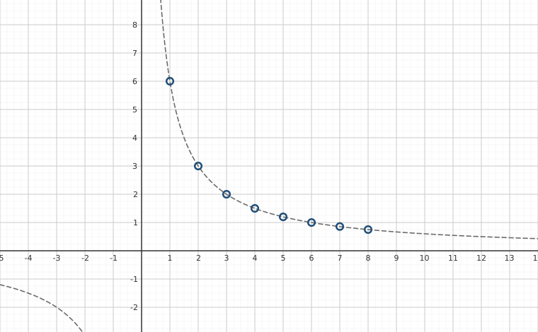
Some remarks about Example 10.1.1 are in order. We first note that since sequences are functions, we can graph them in the same way we graph functions. For example, if we wish to graph the sequence ${b_{k}}_{k = 0}^{\infty}$ from Example 10.1.1, we graph the equation $y = b (k)$ for the values $k greater than or equal to 0$ . That is, we plot the points $(k, b (k))$ for the values of $k$ in the domain, $k equals 0, 1, 2, …$ . The resulting collection of points is the graph of the sequence. Note that we do not connect the dots in a pleasing fashion as we are used to doing, because the domain is just the whole numbers in this case, not a collection of intervals of real numbers.²

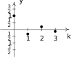
Coordinate-plane figure. — **Figure 10.1**

Graphing $y = b_{k} = \frac{{(- 1)}^{k}}{2 k + 1}$ , $k greater than or equal to 0$

Speaking of ${b_{k}}_{k = 0}^{\infty}$ , the astute and mathematically minded reader will correctly note that this technically isn't a sequence, since according to Definition 10.1, sequences are functions whose domains are the natural numbers, not the whole numbers, as is the case with ${b_{k}}_{k = 0}^{\infty}$ . In other words, to satisfy Definition 10.1, we need to shift the variable $k$ so it starts at $k equals 1$ instead of $k equals 0$ .

To see how we can do this, it helps to think of the problem graphically. What we want is to shift the graph of $y = b (k)$ to the right one unit, and thinking back to Section 5.4, we can accomplish this by replacing $k$ with $k minus 1$ in the definition of ${b_{k}}_{k = 0}^{\infty}$ .

Specifically, let $c_{k} = b_{k - 1}$ where $k minus 1 greater than or equal to 0$ . We get $c_{k} = \frac{{(- 1)}^{k - 1}}{2 (k - 1) + 1} = \frac{{(- 1)}^{k - 1}}{2 k - 1}$ , where now $k greater than or equal to 1$ . We leave to the reader to verify that ${c_{k}}_{k = 1}^{\infty}$ generates the same list of numbers as does ${b_{k}}_{k = 0}^{\infty}$ , but the former satisfies Definition 10.1, while the latter does not.

Like so many things in this text, we acknowledge that this point is pedantic and join the vast majority of authors who adopt a more relaxed view of Definition 10.1 to include any function which generates a list of numbers which can then be matched up with the natural numbers.³

One last note about Example 10.1.1 concerns the manner in which the sequences in numbers and are defined. We say these two sequences are described `recursively.' In each instance, an initial value of the sequence is given which is then followed by a recursion equation a formula which enables us to use known terms of the sequence to determine other terms.

The terms of the sequence from number is given notation and name: $f_{n} = n!$ is called $n$ -factorial. Using the `!' notation, we can describe the factorial sequence as: $0 ! equals 1$ and $n! = n (n - 1)!$ for $n greater than or equal to 1$ .

After $0 ! equals 1$ the next four terms, written out in detail, are $1! = 1 \cdot 0! = 1 \cdot 1 = 1$ , $2! = 2 \cdot 1! = 2 \cdot 1 = 2$ , $3! = 3 \cdot 2! = 3 \cdot 2 \cdot 1 = 6$ and $4! = 4 \cdot 3! = 4 \cdot 3 \cdot 2 \cdot 1 = 24$ . From this, we see a more informal way of computing $n!$ , which is $n! = n \cdot (n - 1) \cdot (n - 2) \dots 2 \cdot 1$ with $0 ! equals 1$ as a special case. (We will study factorials in greater detail in Section 10.4.)⁴

While none of the sequences in Example 10.1.1 worked out to be the sequence in (Equation 10.1), they do give us some insight into what kinds of patterns to look for. Two patterns in particular are given in the next definition.

Definition

Arithmetic and Geometric Sequences: Suppose ${a_{n}}_{n = k}^{\infty}$ is a sequence⁵

If there is a number $d$ so that $a_{n + 1} = a_{n} + d$ for all $n \geq k$ , then ${a_{n}}_{n = k}^{\infty}$ is called an arithmetic sequence. The number $d$ is called the common difference.
If there is a number $r$ so that $a_{n + 1} = r a_{n}$ for all $n \geq k$ , then ${a_{n}}_{n = k}^{\infty}$ is called a geometric sequence. The number $r$ is called the common ratio.

In English, an arithmetic sequence is one in which we proceed from one term to the next by always adding the fixed number $d$ . If this sort of `constant change' idea sounds familiar, it should. Indeed, arithmetic sequences are merely linear functions, something we will explore in more detail shortly. Note the name `common difference' comes from a slight rewrite of the recursion equation from $a_{n + 1} = a_{n} + d$ to $a_{n + 1} - a_{n} = d$ . That is, every pair of successive terms has the same or common difference, $d$ .

Analogously, a geometric sequence is one in which we proceed from one term to the next by always multiplying by the same fixed number $r$ . If this notion sounds familiar, it is because geometric sequences are, in fact, exponential functions. Again, we will explore this connection in more detail later. We note that if $a sub n not equal to 0$ , we can rearrange the recursion equation to get $\frac{a_{n + 1}}{a_{n}} = r$ . Hence, every pair of successive terms has the same or common ratio, $r$ .

Some sequences are arithmetic, some are geometric and some are neither as the next example illustrates.⁶

Example 2

Determine if the following sequences are arithmetic, geometric or neither. If arithmetic, find the common difference $d$ ; if geometric, find the common ratio $r$ .

$a_{n} = \frac{5^{n - 1}}{3^{n}}$ , $n greater than or equal to 1$
$b_{k} = \frac{{(- 1)}^{k}}{2 k + 1}$ , $k greater than or equal to 0$
${2 n - 1}_{n = 1}^{\infty}$
$\frac{1}{2}, - \frac{3}{4}, \frac{9}{8}, - \frac{27}{16}, \dots$

A good rule of thumb to keep in mind when working with sequences is “When in doubt, write it out!” Writing out the first several terms can help you identify the pattern of the sequence should one exist.

From Example 10.1.1, we know that the first four terms of this sequence are $\frac{1}{3}, \frac{5}{9}, \frac{25}{27}$ and $\frac{125}{81}$ . To see if this is an arithmetic sequence, we look at the successive differences of terms. We find that $a_{2} - a_{1} = \frac{5}{9} - \frac{1}{3} = \frac{2}{9}$ and $a_{3} - a_{2} = \frac{25}{27} - \frac{5}{9} = \frac{10}{27}$ . Since we get different numbers, there is no `common difference' and we have established that the sequence is not arithmetic.
To see if the sequence is geometric, we compute the ratios of successive terms. The first three ratios suggest the sequence is geometric:
$\frac{a_{2}}{a_{1}} = \frac{\frac{5}{9}}{\frac{1}{3}} = \frac{5}{3}, \frac{a_{3}}{a_{2}} = \frac{\frac{25}{27}}{\frac{5}{9}} = \frac{5}{3} and \frac{a_{4}}{a_{3}} = \frac{\frac{125}{81}}{\frac{25}{27}} = \frac{5}{3}$
To prove the sequence is geometric, however, we must show that $\frac{a_{n + 1}}{a_{n}} = r$ for all $n$ :
$\frac{a_{n + 1}}{a_{n}} = \frac{\frac{5^{(n + 1) - 1}}{3^{n + 1}}}{\frac{5^{n - 1}}{3^{n}}} = \frac{5^{n}}{3^{n + 1}} \cdot \frac{3^{n}}{5^{n - 1}} = \frac{5}{3}$
Hence, the sequence is geometric with common ratio $r = \frac{5}{3}$ .
Again, we have Example 10.1.1 to thank for providing the first four terms of this sequence: $1, - \frac{1}{3}, \frac{1}{5}$ and $- \frac{1}{7}$ . We find $b_{1} - b_{0} = - \frac{4}{3}$ and $b_{2} - b_{1} = \frac{8}{15}$ . Hence, the sequence is not arithmetic. To see if it is geometric, we compute $\frac{b_{1}}{b_{0}} = - \frac{1}{3}$ and $\frac{b_{2}}{b_{1}} = - \frac{3}{5}$ . Since there is no `common ratio,' we conclude the sequence is not geometric, either.
As we saw in Example 10.1.1, the sequence ${2 n - 1}_{n = 1}^{\infty}$ generates the odd numbers: $1, 3, 5, 7, …$ . Computing the first few differences, we find $a_{2} - a_{1} = 2$ , $a_{3} - a_{2} = 2$ , and $a_{4} - a_{3} = 2$ . This suggests that the sequence is arithmetic. To prove this is the case, we find
$a_{n + 1} - a_{n} = (2 (n + 1) - 1) - (2 n - 1) = 2 n + 2 - 1 - 2 n + 1 = 2$
This establishes that the sequence is arithmetic with common difference $d equals 2$ . To see if it is geometric, we compute $\frac{a_{2}}{a_{1}} = 3$ and $\frac{a_{3}}{a_{2}} = \frac{5}{3}$ . Since these ratios are different, we conclude the sequence is not geometric.
We met our last sequence at the beginning of the section. Given that $a_{2} - a_{1} = - \frac{5}{4}$ and $a_{3} - a_{2} = \frac{15}{8}$ , the sequence is not arithmetic. Computing the first few ratios, however, gives us $\frac{a_{2}}{a_{1}} = - \frac{3}{2}$ , $\frac{a_{3}}{a_{2}} = - \frac{3}{2}$ and $\frac{a_{4}}{a_{3}} = - \frac{3}{2}$ . Since these are the only terms given to us, we assume that the pattern of ratios continue in this fashion and conclude that the sequence is geometric.

We are now one step away from determining an explicit formula for the sequence given in (Equation 10.1). We know that it is a geometric sequence and our next result gives us the explicit formula we require.

Equation

Formulas for Arithmetic and Geometric Sequences:

An arithmetic sequence with first term $a sub 1 equals a$ and common difference $d$ is given by
$a_{n} = a + (n - 1) d, n \geq 1$
A geometric sequence with first term $a sub 1 equals a$ and common ratio $r not equal to 0$ is given by
$a_{n} = a r^{n - 1}, n \geq 1$

An intuitive way to arrive at Equation 10.1 appeals to Definition 10.2 directly. Given an arithmetic sequence with first term $a$ and common difference $d$ , the way we get from one term to the next is by adding $d$ . Hence, the terms of the sequence are: $a$ , $a + d$ , $a plus 2 ⁢ d$ , $a plus 3 ⁢ d$ , …. We see that to reach the $n$ th term, we add $d$ to $a$ exactly $open parenthesis n minus 1 close parenthesis$ times, which is exactly what the formula says.⁷

Note if we rewrite the formula $a_{n} = a_{1} + (n - 1) d$ using traditional function notation as $a (n) = a (1) + d (n - 1)$ we can see arithmetic sequences are linear functions.⁸ Indeed, relabeling the function $a$ as ` $f$ ' and the independent variable $n$ as ` $x$ ,' we can make the identifications $x sub 0 equals 1$ , and $m = d$ so as to put the equation $a (n) = a (1) + d (n - 1)$ into the form of Equation 1.1:

$\begin{matrix} a (n) & = & a (1) & + & d (n - 1) \\ f (x) & = & f (1) & + & m (x - 1) \end{matrix}$

Hence, arithmetic sequences are linear functions with slope $d$ whose domains are the natural numbers.

The derivation of the formula for geometric series follows similarly. Here, we start with the first term $a$ and go from one term to the next by multiplying by $r$ . We get $a, a r, a r^{2}, a r^{3}$ and so forth. The $n$ th term results from multiplying $a$ by $r$ exactly $open parenthesis n minus 1 close parenthesis$ times.⁹

In the same way arithmetic sequences are linear functions, geometric sequences are exponential functions. Writing $a_{n} = a_{1} r^{n - 1}$ as $a (n) = a (1) r^{n - 1}$ , we can relabel $a$ as $f$ and $n$ as $x$ and make the identifications $x sub 0 equals 1$ and $b = r$ to put the equation into the form described in Definition 7.2:

$\begin{matrix} a (n) & = & a (1) r^{n - 1} \\ f (x) & = & f (1) b^{x - 1} \end{matrix}$

So, geometric sequences are exponential functions with base $r$ whose domains are the natural numbers.

With Equation 10.1 in place, we finally have the tools required to find an explicit formula for the $n$ th term of the sequence given in (Equation 10.1). We know from Example 10.1.2 that it is geometric with common ratio $r = - \frac{3}{2}$ . The first term is $a = \frac{1}{2}$ so by Equation 10.1 we get $a_{n} = a r^{n - 1} = \frac{1}{2} {(- \frac{3}{2})}^{n - 1}$ for $n greater than or equal to 1$ . After a touch of simplifying, we get $a_{n} = \frac{{(- 3)}^{n - 1}}{2^{n}}$ for $n greater than or equal to 1$ . Note that we can easily check our answer by substituting in values of $n$ and seeing that the formula generates the sequence given in (Equation 10.1). We leave this to the reader. In particular, the 117th term in the sequence is $a_{117} = \frac{1}{2} {(- \frac{3}{2})}^{117 - 1} = \frac{3^{116}}{2^{117}}$ .

Our next example gives us more practice finding patterns.

Example 3

Find an explicit formula for the $n^{th}$ term of the following sequences.

$0.9, 0.09, 0.009, 0.0009, …$
$\frac{2}{5}, 2, - \frac{2}{3}, - \frac{2}{7}, \dots$
$1, - \frac{2}{7}, \frac{4}{13}, - \frac{8}{19}, \dots$

Although this sequence may seem strange, the reader can verify it is actually a geometric sequence with common ratio $r = 0.1 = \frac{1}{10}$ . With $a = 0.9 = \frac{9}{10}$ , we get $a_{n} = \frac{9}{10} {(\frac{1}{10})}^{n - 1}$ for $n greater than or equal to 0$ . Simplifying, we get $a_{n} = \frac{9}{10^{n}}$ , $n greater than or equal to 1$ . There is more to this sequence than meets the eye and we shall return to this example in the next section.
As the reader can verify, this sequence is neither arithmetic nor geometric. In an attempt to find a pattern, we rewrite the second term with a denominator to make all the terms appear as fractions and associate the `' with the denominators so we have a constant numerator:
$\frac{2}{5}, \frac{2}{1}, \frac{2}{- 3}, - \frac{2}{- 7}, \dots$
This tells us that we can tentatively sketch out the formula for the sequence as $a_{n} = \frac{2}{D_{n}}$ where $D_{n}$ is the sequence of denominators.
The sequence of the denominators: $5, 1, - 3, - 7, \dots$ is seen to be an arithmetic sequence with a common difference of $minus 4$ . Using Equation 10.1 with $a equals 5$ and $d = - 4$ , we get the $n$ th denominator by the formula $D_{n} = 5 + (n - 1) (- 4) = 9 - 4 n$ for $n greater than or equal to 1$ . Hence, our final answer is $a_{n} = \frac{2}{9 - 4 n}$ , $n greater than or equal to 1$ .
The sequence as given is neither arithmetic nor geometric, so we proceed as in the last problem to try to get patterns individually for the numerator and denominator. Letting $C_{n}$ and $D_{n}$ denote the sequence of numerators and denominators, respectively, so that $a_{n} = \frac{C_{n}}{D_{n}}$ .
After some experimentation,¹⁰ we choose to write the first term as a fraction and associate the negatives `' with the numerators. This yields
$\frac{1}{1}, \frac{- 2}{7}, \frac{4}{13}, \frac{- 8}{19}, \dots$
The numerators form the sequence $1, - 2, 4, - 8, \dots$ which is geometric with $a equals 1$ and $r = - 2$ , so we get $C_{n} = {(- 2)}^{n - 1}$ , for $n greater than or equal to 1$ .
The denominators $1, 7, 13, 19, …$ form an arithmetic sequence with $a equals 1$ and $d equals 6$ . Hence, we get $D_{n} = 1 + 6 (n - 1) = 6 n - 5$ , for $n greater than or equal to 1$ .
Putting these two formulas together, we obtain our formula for $a_{n} = \frac{C_{n}}{D_{n}} = \frac{{(- 2)}^{n - 1}}{6 n - 5}$ , for $n greater than or equal to 1$ . We leave it to the reader to show that this checks out.

While the last problem in Example 10.1.3 was neither geometric nor arithmetic, it did resolve into a combination of these two kinds of sequences. If handed the sequence $2, 5, 10, 17, …$ , we would be hard-pressed to find a formula for $a_{n}$ if we restrict our attention to these two archetypes. We said before that there is no general algorithm for finding the explicit formula for the $n$ th term of a given sequence, and it is only through experience gained from evaluating sequences from explicit formulas that we learn to begin to recognize number patterns.

The pattern $1, 4, 9, 16, …$ is rather recognizable as the squares, so the formula $a_{n} = n^{2}$ , $n greater than or equal to 1$ may not be too hard to determine. With this in mind, it's possible to see $2, 5, 10, 17, …$ as the sequence $1 + 1, 4 + 1, 9 + 1, 16 + 1, \dots$ , so that $a_{n} = n^{2} + 1$ , $n greater than or equal to 1$ .

Of course, since we are given only a small sample of the sequence, we shouldn't be too disappointed to find out this isn't the only formula which generates this sequence. For example, consider the sequence defined by $b_{n} = - \frac{1}{4} n^{4} + \frac{5}{2} n^{3} - \frac{31}{4} n^{2} + \frac{25}{2} n - 5$ , $n greater than or equal to 1$ . The reader is encouraged to verify that it also produces the terms $2, 5, 10, 17$ . In fact, it can be shown that given any finite sample of a sequence, there are infinitely many explicit formulas all of which generate those same finite points. This means that there will be infinitely many correct answers to some of the exercises in this section.¹¹ Just because your answer doesn't match ours doesn't mean it's wrong. As always, when in doubt, write your answer out. As long as it produces the same terms in the same order as what the problem wants, your answer is correct.

Sequences play a major role in the Mathematics of Finance, as we have already seen with Equation 7.2 in Section 7.6. Recall that if we invest $P$ dollars at an annual percentage rate $r$ and compound the interest $n$ times per year, the formula for $A_{k}$ , the amount in the account after $k$ compounding periods, is $A_{k} = P {(1 + \frac{r}{n})}^{k} = [P (1 + \frac{r}{n})] {(1 + \frac{r}{n})}^{k - 1}$ , $k greater than or equal to 1$ . We leave it to the reader to show this is a geometric sequence with first term $P (1 + \frac{r}{n})$ and common ratio $(1 + \frac{r}{n})$ .

In section 7.6, we showed $lim_{n \to \infty} P {(1 + \frac{r}{n})}^{n t} = P e^{r t}$ , where we noted, at the time, that the limit here was taken on a discrete, rather than continuous variable. That didn't stop us from using the limit properties listed in Theorem 6.2. We talk more on the limits of sequences next.

Limits of Sequences

Consider the sequence $a_{n} = \frac{3 n}{n + 1}$ , $n greater than or equal to 1$ . Suppose we wished to find $lim n → ∞ a sub n$ .

We should first note that even though the domain of the sequence $a_{n}$ is discrete, we can nonetheless discuss what happens as $n → ∞$ since for any real number $M greater than 0$ , we can find a natural number $n > M$ . (We could, for instance take $n = ⌊ M ⌋ + 1$ .)

Next, note that we can visualize the sequence $a_{n} = \frac{3 n}{n + 1}$ , $n greater than or equal to 1$ as being points on the graph of $f (x) = \frac{3 x}{x + 1}$ :

Image: sequenceoncurve — **Figure 10.2**

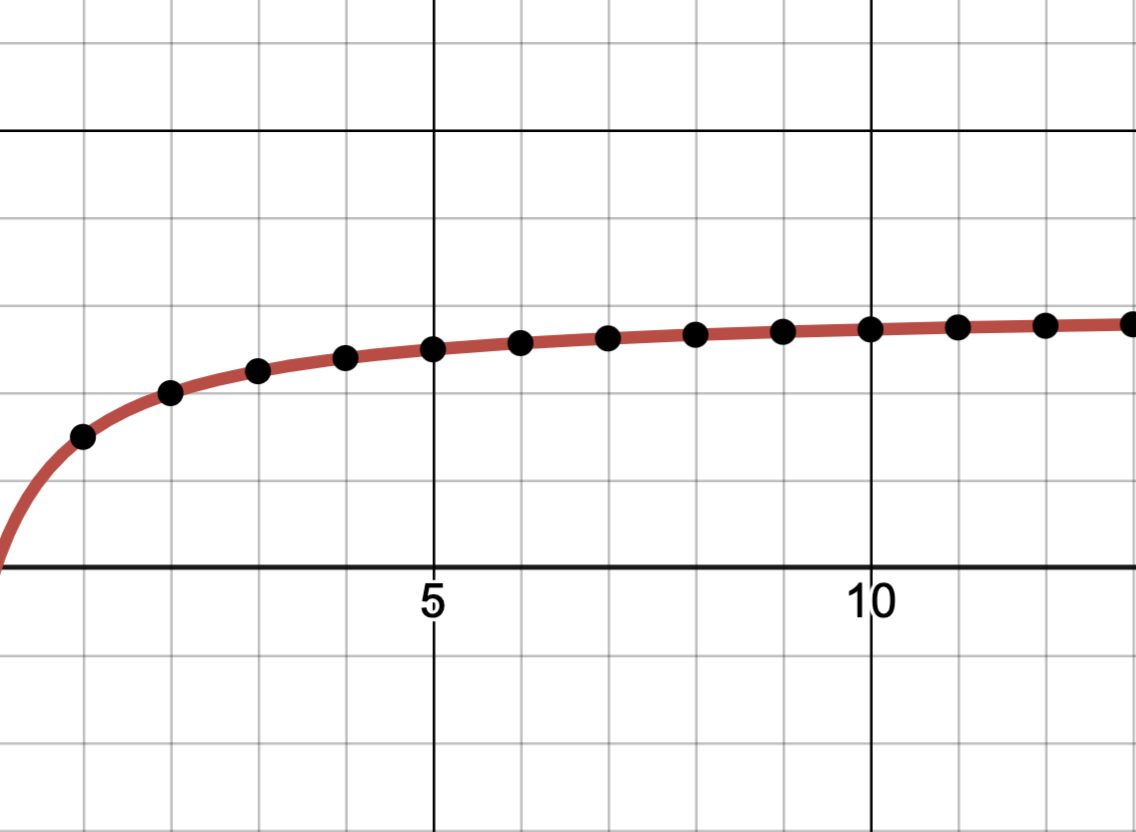
Comparing leading terms of numerator and denominator, as $x → ∞$ , $\frac{3 x}{x + 1} \approx \frac{3 x}{x} = 3$ . Hence, $lim x → ∞$ $\frac{3 x}{x + 1} = 3$ , which means all of the $y$ -values on the graph of $y = f (x)$ , including the $y$ -values of the graph of the sequence, approach $3$ as $x → ∞$ . It stands to reason, then that $lim n → ∞$ $\frac{3 n}{n + 1} = 3$ .

The long and short of the above argument is that since $lim x → ∞$ $\frac{3 x}{x + 1}$ exists, $lim n → ∞$ $\frac{3 n}{n + 1} =$ $lim x → ∞$ $\frac{3 x}{x + 1}$ . While the syntax of ` $lim n → ∞$ $\frac{3 n}{n + 1} =$ $lim x → ∞$ $\frac{3 x}{x + 1}$ ' appears to be just a switch in a dummy variable,¹² the switch from ` $n$ ' to ` $x$ ' indicates switching from a discrete variable to a continuous one. This sort of maneuver is called passing to a continuous variable and is one of the primary ways we can use what we've already studied to analyze limits of sequences.

Theorem

If $lim x → ∞ f ⁢ open parenthesis x close parenthesis equals L$ and $f (n) = a_{n}$ for all $n \geq k$ for some natural number $k$ , then $lim n → ∞ a sub n equals L$ .

Note the phrase ` $f (n) = a_{n}$ for all $n \geq k$ for some natural number $k$ ' indicates the focus on what is happening as $n → ∞$ . In other words, the first finitely many sequence values do not impact the value of $lim n → ∞ a sub n$ . We are just concerned with the long-run or end behavior here. The reason Theorem 10.1 works, indeed why all of the limit properties discussed in Section 6.1 work with sequences as well as functions of continuous variables is because the formal definitions associated with limits of both sequences and functions share the same mathematical `bones.' (See a Calculus instructor for more details.) We'll explore these connections more deeply in the Exercises.

We have special words to describe sequences which have limits and those which do not.

Definition

If ${a_{n}}$ is a sequence and $lim n → ∞ a sub n equals L$ , we say the sequence ${a_{n}}$ converges to $L$ . If $lim n → ∞ a sub n$ does not exist, we say the sequence diverges.

Example 4

Determine the following limits by passing to a continuous variable. Check your answers graphically.
1. $lim n → ∞$ $\frac{1 - n^{2}}{2 n^{2} - 3 n + 1}$ .
2. $lim_{n \to \infty} n e^{- 2 n}$ .
What difficulties do you encounter when trying to pass the limit $lim n → ∞$ $\frac{{(- 1)}^{n}}{n^{2} + 1}$ to a continuous variable? What appears to be the limit?

1. Passing $lim n → ∞$ $\frac{1 - n^{2}}{2 n^{2} - 3 n + 1}$ to a continuous variable gives $lim x → ∞$ $\frac{1 - x^{2}}{2 x^{2} - 3 x + 1}$ . Comparing leading terms, we have that as $x → ∞$ , $\frac{1 - x^{2}}{2 x^{2} - 3 x + 1} \approx \frac{- x^{2}}{2 x^{2}} = - \frac{1}{2}$ , so $lim x → ∞$ $\frac{1 - x^{2}}{2 x^{2} - 3 x + 1} = - \frac{1}{2}$ . By Theorem 10.1, $lim n → ∞$ $\frac{1 - n^{2}}{2 n^{2} - 3 n + 1} = - \frac{1}{2}$ . This tracks given the graph below on the left.
2. Passing $lim_{n \to \infty} n e^{- 2 n}$ to a continuous variable gives $lim_{x \to \infty} x e^{- 2 x}$ . Here we do not have leading terms to compare - but we do have an indeterminate form ` $∞ times 0$ ', That being said, as discussed following Example 7.4.5 in Section 7.4, the factor $e^{- 2 x}$ will dominate the factor $x$ as $x → ∞$ , so we have $lim_{n \to \infty} n e^{- 2 n} = lim_{x \to \infty} x e^{- 2 x} = 0$ . The graph below on the right confirms this.
  Figure 10.3
  Figure 10.4
  $a_{n} = \frac{1 - n^{2}}{2 n^{2} - 3 n + 1}$ along with $y = \frac{1 - x^{2}}{2 x^{2} - 3 x + 1}$
  $a_{n} = n e^{- 2 n}$ along with $y = x e^{- 2 x}$
When passing $lim n → ∞$ $\frac{{(- 1)}^{n}}{n^{2} + 1}$ to a continuous variable, we get the factor ${(- 1)}^{x}$ which is non-real for several¹³ real numbers such as $x = \frac{1}{2}$ , $x equals 117.23$ , or $x equals 3000 ⁢ π$ . That being said, we note that the factor ${(- 1)}^{n}$ alternates the sign of each term: $open parenthesis plus close parenthesis ⁢ 1$ if $n$ is even and $minus 1$ if $n$ is odd: $- \frac{1}{2}, \frac{1}{5}, - \frac{1}{10}, \frac{1}{17}, \dots$ .
This means that we can bound the sequence we're interested in between two other sequences we know something about: $- \frac{1}{n^{2} + 1} \leq \frac{{(- 1)}^{n}}{n^{2} + 1} \leq \frac{1}{n^{2} + 1}$ .
Passing to a continuous variable, $lim n → ∞$ $- \frac{1}{n^{2} + 1} =$ $lim x → ∞$ $- \frac{1}{x^{2} + 1} = 0$ and $lim n → ∞$ $\frac{1}{n^{2} + 1} =$ $lim x → ∞$ $\frac{1}{x^{2} + 1} = 0$ , so it stands to reason that $lim n → ∞$ $\frac{{(- 1)}^{n}}{n^{2} + 1} = 0$ as well. We sketch the situation out below.
Figure 10.5

The sequence in number in Example 10.1.4 is an example of an alternating sequence, so-named because the terms alternate in sign. Alternating sequences play a large role in the study of infinite series (whatever those are) in Calculus,¹⁴ so it is worth pointing them out here.

Next, the reasoning we used to determine $lim n → ∞$ $\frac{{(- 1)}^{n}}{n^{2} + 1} = 0$ is sound and is codified in the following theorem. We state the result for both sequences (discrete functions) and (continuous) functions.

Theorem

The Squeeze Theorem:

Suppose for some natural number $k$ , $b_{n} \leq a_{n} \leq c_{n}$ for all $n \geq k$ .
If $lim_{n \to \infty} b_{n} = lim_{n \to \infty} c_{n} = L$ , then $lim n → ∞ a sub n equals L$ .
Suppose for some real number $M$ , $g (x) \leq f (x) \leq h (x)$ for all $x \geq M$ .
If $lim_{x \to \infty} g (x) = lim_{x \to \infty} h (x) = L$ , then $lim x → ∞ f ⁢ open parenthesis x close parenthesis equals L$ .

The Squeeze Theorem is so-named because the two sequences (functions) which bound the middle sequence (function) `squeeze' the middle function to the common limit, $L$ .

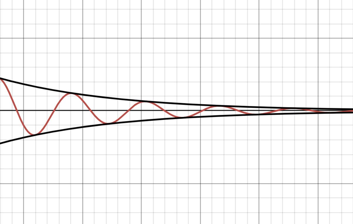
The graph of $y = f (x)$ being `squeezed' to a common limit by the graphs of $y = g (x)$ and $y = h (x)$ .

Passing to a continuous variable in conjunction with the Squeeze Theorem can be used to prove certain classes of Geometric Sequences converge. We have the following:

Theorem

Limits of Geometric Sequences: Given a geometric sequence with common ratio $r$ :

If $minus 1 less than r less than 1$ , the sequence converges to $0$ .
If $r equals 1$ , the sequence converges to the first term, $a$ .
If $r greater than 1$ or $r less than or equal to minus 1$ , the sequence diverges.

We encourage the reader to think through each of the cases stated in Theorem 10.3 to make sure the conclusions seem reasonable. We'll have occasion to cite Theorem 10.3 in the next section. For now, it's time for some Exercises.

Exercises

In Exercises -, write out the first four terms of the given sequence.

$a_{n} = 2^{n} - 1$ , $n greater than or equal to 0$
$d_{j} = {(- 1)}^{\frac{j (j + 1)}{2}}$ , $j greater than or equal to 1$
${5 k - 2}_{k = 1}^{\infty}$
${\frac{n^{2} + 1}{n + 1}}_{n = 0}^{\infty}$
${\frac{x^{n}}{n^{2}}}_{n = 1}^{\infty}$
${\frac{\ln (n)}{n}}_{n = 1}^{\infty}$
$a sub 1 equals 3$ , $a_{n + 1} = a_{n} - 1$ , $n greater than or equal to 1$
$d sub 0 equals 12$ , $d_{m} = \frac{d_{m - 1}}{100}$ , $m greater than or equal to 1$
$b sub 1 equals 2$ , $b_{k + 1} = 3 b_{k} + 1$ , $k greater than or equal to 1$
$c_{0} = - 2$ , $c_{j} = \frac{c_{j - 1}}{(j + 1) (j + 2)}$ , $j greater than or equal to 1$
$a sub 1 equals 117$ , $a_{n + 1} = \frac{1}{a_{n}}$ , $n greater than or equal to 1$
$s sub 0 equals 1$ , $s_{n + 1} = x^{n + 1} + s_{n}$ , $n greater than or equal to 0$
$F sub 0 equals 1$ , $F sub 1 equals 1$ , $F_{n} = F_{n - 1} + F_{n - 2}$ , $n greater than or equal to 2$ (This is the famous Fibonacci Sequence )

In Exercises - determine if the given sequence is arithmetic, geometric or neither. If it is arithmetic, find the common difference $d$ ; if it is geometric, find the common ratio $r$ .

${3 n - 5}_{n = 1}^{\infty}$
$a_{n} = n^{2} + 3 n + 2$ , $n greater than or equal to 1$
$\frac{1}{3}$ , $\frac{1}{6}$ , $\frac{1}{12}$ , $\frac{1}{24}$ , …
${3 {(\frac{1}{5})}^{n - 1}}_{n = 1}^{\infty}$
$17$ , $5$ , $minus 7$ , $minus 19$ , …
$2$ , $22$ , $222$ , $2222$ , …
$0.9$ , $9$ , $90$ , $900$ , …
$a_{n} = \frac{n!}{2}$ , $n greater than or equal to 0$ .

In Exercises -, find an explicit formula for the $n^{th}$ term of the given sequence.¹⁵

$3$ , $5$ , $7$ , $9$ , …
$1$ , $- \frac{1}{2}$ , $\frac{1}{4}$ , $- \frac{1}{8}$ , …
$1$ , $\frac{2}{3}$ , $\frac{4}{5}$ , $\frac{8}{7}$ , …
$1$ , $\frac{2}{3}$ , $\frac{1}{3}$ , $\frac{4}{27}$ , …
$1$ , $\frac{1}{4}$ , $\frac{1}{9}$ , $\frac{1}{16}$ , …
$x$ , $- \frac{x^{3}}{3}$ , $\frac{x^{5}}{5}$ , $- \frac{x^{7}}{7}$ , …
$0.9, 0.99, 0.999, 0.9999, …$
$27, 64, 125, 216, …$
$1, 0, 1, 0, …$

In Exercises -, find the indicated limit by using Theorem 10.1 and passing to a continuous variable.¹⁶

$lim n → ∞$ $\frac{2 n^{2} - 3 n + 1}{4 - n^{2}}$
$lim k → ∞$ $\frac{k^{2} + 7 k - 3}{3 k - k^{3}}$
$lim m → ∞$ $\frac{117 m^{42} + 3 m + 1}{e^{2 m} + 6}$

In Exercises -, use the Squeeze Theorem, Theorem 10.2 to help you determine the limit.¹⁷

$lim n → ∞$ $\frac{{(- 1)}^{n}}{3 n + 1}$
$lim k → ∞$ $1 - {(- \frac{2}{3})}^{k}$
$lim m → ∞$ $\frac{{(- 1)}^{\frac{m^{2} - m}{2}}}{m!}$
Find a sequence which is both arithmetic and geometric. (Hint: Start with $a_{n} = c$ for all $n$ .)
Show that a geometric sequence can be transformed into an arithmetic sequence by taking the natural logarithm of the terms.
Thomas Robert Malthus is credited with saying, “The power of population is indefinitely greater than the power in the earth to produce subsistence for man. Population, when unchecked, increases in a geometrical ratio. Subsistence increases only in an arithmetical ratio. A slight acquaintance with numbers will show the immensity of the first power in comparison with the second.” (See this webpage for more information.) Discuss this quote with your classmates from a sequences point of view.
This classic problem involving sequences shows the power of geometric sequences. Suppose that a wealthy benefactor agrees to give you one penny today and then double the amount she gives you each day for 30 days. So, for example, you get two pennies on the second day and four pennies on the third day. How many pennies do you get on the $30 to the power th$ day? What is the total dollar value of the gift you have received?
Research the terms `arithmetic mean' and `geometric mean.' With the help of your classmates, show that a given term of a arithmetic sequence $a_{k}$ , $k greater than or equal to 2$ is the arithmetic mean of the term immediately preceding, $a sub k ⁢ minus 1$ it and immediately following it, $a sub k ⁢ plus 1$ . State and prove an analogous result for geometric sequences.
Discuss with your classmates how the results of this section might change if we were to examine sequences of other mathematical things like complex numbers or matrices. Find an explicit formula for the $n^{th}$ term of the sequence $i, - 1, - i, 1, i, \dots$ . List out the first four terms of the matrix sequences we discussed in Exercise in Section 9.3.

Answers

$0, 1, 3, 7$
$- 1, - 1, 1, 1$
$3, 8, 13, 18$
$1, 1, \frac{5}{3}, \frac{5}{2}$
$x, \frac{x^{2}}{4}, \frac{x^{3}}{9}, \frac{x^{4}}{16}$
$0, \frac{\ln (2)}{2}, \frac{\ln (3)}{3}, \frac{\ln (4)}{4}$
$3, 2, 1, 0$
$12, 0.12, 0.0012, 0.000012$
$2, 7, 22, 67$
$- 2, - \frac{1}{3}, - \frac{1}{36}, - \frac{1}{720}$
$117, \frac{1}{117}, 117, \frac{1}{117}$
$1, x + 1, x^{2} + x + 1, x^{3} + x^{2} + x + 1$
$1, 1, 2, 3$
arithmetic, $d equals 3$
neither
geometric, $r = \frac{1}{2}$
geometric, $r = \frac{1}{5}$
arithmetic, $d = - 12$
neither
geometric, $r equals 10$
neither
$a_{n} = 1 + 2 n, n \geq 1$
$a_{n} = {(- \frac{1}{2})}^{n - 1}, n \geq 1$
$a_{n} = \frac{2^{n - 1}}{2 n - 1}, n \geq 1$
$a_{n} = \frac{n}{3^{n - 1}}, n \geq 1$
$a_{n} = \frac{1}{n^{2}}, n \geq 1$
$\frac{{(- 1)}^{n - 1} x^{2 n - 1}}{2 n - 1}, n \geq 1$
$a_{n} = \frac{10^{n} - 1}{10^{n}}, n \geq 1$
$a_{n} = {(n + 2)}^{3}, n \geq 1$
$a_{n} = \frac{1 + {(- 1)}^{n - 1}}{2}, n \geq 1$
$lim n → ∞$ $\frac{2 n^{2} - 3 n + 1}{4 - n^{2}} = - 2$
$lim k → ∞$ $\frac{k^{2} + 7 k - 3}{3 k - k^{3}} = 0$
$lim m → ∞$ $\frac{117 m^{42} + 3 m + 1}{e^{2 m} + 6} = 0$
$lim n → ∞$ $\frac{{(- 1)}^{n}}{3 n + 1} = 0$
$lim k → ∞$ $1 - {(- \frac{2}{3})}^{k} = 1$
$lim m → ∞$ $\frac{{(- 1)}^{\frac{m^{2} - m}{2}}}{m!} = 0$

Recall that this is the set $ℕ equals open brace 1, 2, 3, … close brace$ . ↩
If you feel a sense of nostalgia, you should see Section 1.1. ↩
We're basically talking about the `countably infinite' subsets of the real number line when we do this. ↩
Another famous sequence, the Fibonacci Numbers are defined also recursively and are explored in the exercises. ↩
Note that we have adjusted for the fact that not all `sequences' begin at $n equals 1$ . ↩
Can a sequence be both arithmetic and geometric? See Exercise . ↩
We formalize this argument in Section 10.3. ↩
Note here $a$ is a function, so the expressions $a (n)$ and $a ⁢ open parenthesis 1 close parenthesis$ here represent the outputs from $a$ . On the other hand, the expression $d ⁢ open parenthesis n minus 1 close parenthesis$ indicates multiplication of the real numbers $d$ and $open parenthesis n minus 1 close parenthesis$ . ↩
We note here that the reason $r equals 0$ is excluded from Equation 10.1 is to avoid an instance of $0 to the power 0$ which is an indeterminate form. (See the remarks following Definition 2.1 in Section 2.1.) ↩
Here we take `experimentation' to mean a frustrating guess-and-check session. ↩
For more on this, see When Every Answer is Correct: Why Sequences and Number Patterns Fail the Test . ↩
which it would be without context ↩
Actually, `uncountably infinite' … ↩
We'll touch on these in the next section, too. ↩
Use the formulas in Equation 10.1 as needed. ↩
See Example 10.1.4. ↩
See part of Example 10.1.4. ↩

Adapted from Precalculus, Preliminary 4th Edition (integrated calculus), by Carl Stitz and Jeff Zeager (stitz-zeager.com), licensed under CC BY-NC-SA 3.0. Changes were made: reformatted as an accessible XYZ web edition. License: CC-BY-NC-SA-3.0.