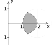
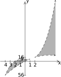
With few exceptions, we have spent our time in this course graphing equations relating two variables. In this section, we explore graphing inequalities relating two variables which usually a two-dimensional region in the plane instead of a one dimensional line or curve.1 In our first example, we restrict our attention to looking at regions in the -plane bounded by equations which describe as a function of .
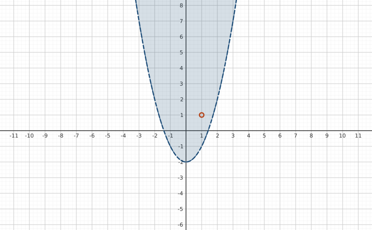
Interactive figureGraphing y > x² − c: shade one side of the curve and test a pointDrag the Vertical offset c, Test point x = a and Test point y = b sliders.
XYZ Graph · viewer build 5edf91b
The inequality y > x² − c describes a region, not a curve: every point strictly above the parabola y = x² − c. The boundary is dashed because the inequality is strict, so points on the parabola are left out, and the shaded region is the inside of the U. The test point (a, b) on its own sliders shows the checking step: drag it into the shading and b > a² − c holds; drag it below the dashed curve and it fails. Slide c and the whole region moves with its boundary.
A few remarks about Example 9.8.1 are in order. First note that each of the regions presented here can be views as graphs of relations as described in Section 5.5. Moreover, there are many ways to describe a region so our answers to number above are by no means unique.
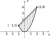
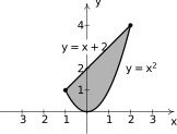
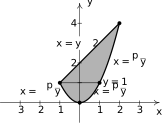
In particular, our solution to number can be visualized as `filling up' the region from the bottom curve, to the top curve, as runs from the leftmost extent of the region at to the rightmost extent at as indicated below. The notion that each determines where to start and stop filling the region is a consequence of us viewing the bounding curves as functions of . That is, for each , we can determine the lower boundary of the region, and the upper boundary of the region, .
Figure 9.29`Filling up' from bottom to top.
Figure 9.30The region .
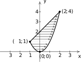
There are times in Calculus where it may be convenient to describe the region as filling up left-to-right as varies from the bottom most extent, to the top most extent, . In this case, we need to describe the bounding curves as functions of . To that end, we solve and for and get three functions of : , and as labeled below.
Figure 9.31`Filling up' from left to right.
Figure 9.32The region
Based on the diagram, we see we need to describe as two pieces. The first piece being bounded on the left by and on the right from to , and the second piece bounded on the left by and on the right by from to . That is,
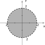
Not all regions in the plane are best described using functions of or .4 Suppose, for instance, we wish to sketch the region Algebraically, we wish to plot all points for which the inequality is true. One way to proceed is to mimic the `sign diagram' routine we use for solving nonlinear inequalities in one variable: rewrite the inequality so as to obtain on one side of the inequality, find the zeros of the non-zero side, choose test values determined by the zeros, and record our solution.
First, we gather all of the terms on one side and leave a on the other: . Next, we find the zeros of the left hand side, that is, where is . Rewriting, we get which describes the circle of radius centered at the origin. In other words, instead of obtaining a few numbers which divide the real number line into intervals, we get an equation of a curve, in this case, a circle, which divides the plane into two regions - the `inside' and `outside' of the circle.
Just like we used test values to determine whether or not an interval belongs to the solution of the inequality, we use test points in the each of the regions to see which of these belong to our solution set.5 We choose to represent the region inside the circle and to represent the points outside of the circle. When we substitute into , we get which is true. This means and all the other points inside the circle are part of the solution. On the other hand, when we substitute into the same inequality, we get which is false. This means along with all other points outside the circle are not part of the solution. What about points on the circle itself? Choosing a point on the circle, say , we get , which means the circle itself does not satisfy the inequality.6 As a result, we leave the circle dashed in the final diagram.
Figure 9.33
The solution to
We put this technique to good use in the following example.
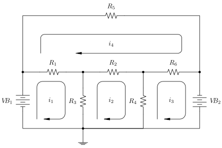
We close this section with a follow-up to Example 9.4.2 in Section 9.4. Recall in the circuit diagrammed below, we have two batteries with source voltages and , measured in volts , along with six resistors with resistances through , measured in kiloohms, .Recall if we think of electrons flowing through the circuit, we can think of the voltage sources as providing the `push' which makes the electrons move, the resistors as obstacles for the electrons to overcome, and the mesh current as a net rate of flow of electrons around the indicated loops.
Figure 9.40
Using Ohm's Law and Kirchhoff's Voltage Law, we can relate the voltage supplied to the circuit by the two batteries to the voltage drops across the six resistors in order to find the four `mesh' currents: , , and , measured in milliamps, . This gives rise to the following system of linear equations:
In Example 9.4.2, we found that under the assumptions , , and all the resistances are all , the mesh currents worked out to be , , , and .
In our final example, we assume and and work to find what combination of resistances would combine to produce these mesh currents.
Exercises
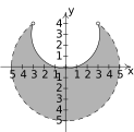
In Exercises -, sketch the solution to each system of nonlinear inequalities in the plane.
Answer
Figure 9.43
Answer
Figure 9.44
Answer
Figure 9.45
Answer
Figure 9.46
Answer
Figure 9.47
Answer
Figure 9.48
Adapted from Precalculus with Integrated Calculus, edition 4i, by Carl Stitz and Jeff Zeager (stitz-zeager.com), licensed under CC BY-NC-SA 3.0. Changes were made: reformatted as an accessible XYZ web edition. License: CC-BY-NC-SA-3.0.
These eBooks are a prerelease and are not yet certified conformant with WCAG 2.1 AA or any other accessibility standard. Every page is built against an automated accessibility gate, and our target for the published editions is WCAG 2.2 Level AA. If something is unusable, please tell us.