In this section, we study systems of non-linear equations. In non-linear equations, we can have variables to powers other than , we can have different variables multiplied together, or variable can occur as arguments of exponential and logarithmic functions.
Unlike the systems of linear equations for which we have developed several algorithmic solution techniques, there is no general algorithm to solve systems of non-linear equations. Moreover, all of the usual hazards of non-linear equations like extraneous solutions and domain restrictions are once again present.
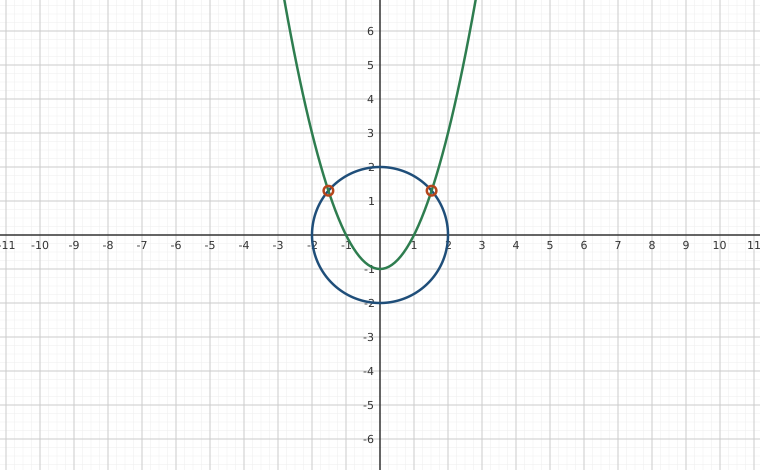
Interactive figureA circle and a parabola: zero, two, three or four common pointsDrag the Radius r and Parabola offset c sliders.
XYZ Graph · viewer build 5edf91b
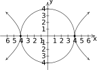
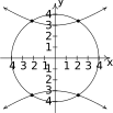
The system is x² + y² = r² together with y = x² − c. Substituting the parabola into the circle gives y² + y + (c − r²) = 0, a quadratic in y whose real roots, when they exist, each produce up to two values of x = ±√(y + c); the marked points are those solutions. Slide the radius r and the offset c to see the count change: a small circle inside the parabola meets it nowhere, a larger one meets it at two points, and the right combination gives four, with three at the instant the circle passes through the vertex. Non-linear systems have no fixed number of solutions, and the picture shows why.
Along with the tried and true techniques of substitution and elimination, we shall often need equal parts tenacity and ingenuity to see a problem through to the end. You may find it necessary to review topics throughout the text which pertain to solving equations involving the various functions we have studied thus far. To get the section rolling we begin with a fairly routine example.
A couple of remarks about Example 9.7.1 are in order. First note that, unlike systems of linear equations, it is possible for a system of non-linear equations to have more than one solution without having infinitely many solutions. In fact, while we characterize systems of nonlinear equations as being `consistent' or `inconsistent,' we generally don't use the labels `dependent' or `independent'.
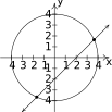
Secondly, as we saw with the last problem, sometimes making a quick sketch of the problem situation can save a lot of time and effort. While in general the curves in a system of non-linear equations may not be easily visualized, it pays to take advantage when they are. Our next example provides some considerable review of many of the topics introduced in this text.
Example 9.7.2 showcases some of the ingenuity and tenacity mentioned at the beginning of the section. Sometimes you just have to look at a system the right way to find the most efficient method to solve it. Sometimes you just have to try something.
Next we explore some common application problems which give rise to systems of nonlinear equations.
One of the important lessons to learn from Example 9.7.3 is that speeds, and more generally, rates, are additive. As we see in our next example, the concept of rate and its associated principles can be applied to a wide variety of problems - not just `distance-rate-time' scenarios.
As is common with `word problems' like Examples 9.7.3 and 9.7.4, there is no short-cut to the answer. Note that in Examples 9.7.3, we formalized the system of non-linear equations before solving whereas in Example 9.7.4, the system remained much in the background. We encourage the reader to carefully think through and apply the basic principles of rate to each (potentially different!) situation. It is time well spent. We also encourage the tracking of units, especially in the early stages of the problem. Not only does this promote uniformity in the units, it also serves as a quick means to check if an equation makes sense.7
Exercises
Exercise idea: follow up on last example and have students formalize the system there using given variables.
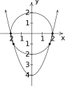
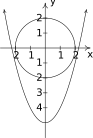
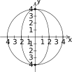
In Exercises -, solve the given system of nonlinear equations. Sketch the graph of both equations on the same set of axes to verify the solution set.
Answer
,
Figure 9.18
Answer
No solution
Figure 9.19
Answer
Figure 9.20
Answer
Figure 9.21
Answer
Figure 9.22
Answer
,
Figure 9.23
In Exercises -, solve the given system of nonlinear equations. Use a graph to help you avoid any potential extraneous solutions.
Answer
Answer
Answer
Answer
Answer
Answer
Answer
Answer
,
Answer
A certain bacteria culture follows the Law of Uninbited Growth, Equation 7.4. After 10 minutes, there are 10,000 bacteria. Five minutes later, there are 14,000 bacteria. How many bacteria were present initially? How long before there are 50,000 bacteria?Answer
Initially, there are bacteria. It will take minutes for the colony to grow to 50,000 bacteria.
Consider the system of nonlinear equations below
If we let and then the system becomes
This associated system of linear equations can then be solved using any of the techniques presented earlier in the chapter to find that and . Thus and .
We say that the original system is linear in form because its equations are not linear but a few substitutions reveal a structure that we can treat like a system of linear equations. Each system in Exercises - is linear in form. Make the appropriate substitutions and solve for and .
Answer
Answer
No solution
Answer
Solve the following system
Answer
Systems of nonlinear equations show up in third semester Calculus in the midst of some really cool problems. The system below came from a problem in which we were asked to find the dimensions of a rectangular box with a volume of 1000 cubic inches that has minimal surface area. The variables , and are the dimensions of the box and is called a Lagrange multiplier. With the help of your classmates, solve the system.8
Answer
According to Theorem 2.18 in Section 2.4, the polynomial can be factored into the product linear and irreducible quadratic factors. In this exercise, we present a method for obtaining that factorization.
Show that has no real zeros.
Because has no real zeros, its factorization must be of the form where each factor is an irreducible quadratic. Expand this quantity and gather like terms together.
Create and solve the system of nonlinear equations which results from equating the coefficients of the expansion found above with those of . You should get four equations in the four unknowns , , and . Write in factored form.
Answer
Factor .Answer
Adapted from Precalculus with Integrated Calculus, edition 4i, by Carl Stitz and Jeff Zeager (stitz-zeager.com), licensed under CC BY-NC-SA 3.0. Changes were made: reformatted as an accessible XYZ web edition. License: CC-BY-NC-SA-3.0.
These eBooks are a prerelease and are not yet certified conformant with WCAG 2.1 AA or any other accessibility standard. Every page is built against an automated accessibility gate, and our target for the published editions is WCAG 2.2 Level AA. If something is unusable, please tell us.