
4.2 Power Functions
Monomial, and, more generally, Laurent monomial functions are specific examples of a much larger class of functions called power functions, as defined below.
Definition 4.2 broadens our scope of functions to include non-integer exponents such as , and . Our primary aim in this section is to ascribe meaning to these quantities.
Rational Number Exponents
The road to real number exponents starts by defining rational number exponents.
There are quite a few items worthy of note which are consequences of Definition 4.3. First off, if is an integer, then so expressions like are synonymous with , as we would expect.3 Second, the definition of can be taken as just and shown to be equal to (or vice-versa) courtesy of properties of radicals. We state both in Definition 4.3 to allow for the reader to choose whichever form is more convenient in a given situation. The critical point to remember is no matter which representation you choose, keep in mind the restrictions if is even, and if , .
Moreover, per this definition, , so we may rewrite principal roots as exponents: and . This makes sense from an algebraic standpoint since per Theorem 4.2, . Hence if we were to assign an exponent notation to , say , then . If the properties of exponents are to hold, then, necessarily, , so or . While this argument helps motivate the notation, as we shall see shortly, great care must be exercised in applying exponent properties in these cases. The long and short of this is that root functions as defined in Section 4.1 are all members of the `power functions' family.
Another important item worthy of note in Definition 4.3 is that it is absolutely essential we express the rational number in lowest terms before applying the root-power definition. For example, consider . Expressing in lowest terms, we get: . Hence, or , either of which is defined for all real numbers . In contrast, consider the equivalence . Here, the expression is defined only for owing to the presence of the even indexed root, . Hence, unless . On the other hand, the expression is defined for all numbers, , since for all . In fact, it can be shown that for all real numbers. This means . So, to review, in general we have: , but unless . Once again the easiest way to avoid confusion here is to reduce the exponent to lowest terms before converting it to root-power notation.
Likewise, we have to be careful about the properties of exponents when it comes to rational exponents. Consider, for instance, the product rule for integer exponents: . Consider and . In the first case, only for . In the second case, for all real numbers . Even though for , and are different functions since they have different domains.
Similarly, the power rule for integer exponents: does not hold in general for rational exponents. To see this, consider the three functions: , , and . In the first case, for only (this is the same function above.) In the second case, the rational number , so for all real numbers, (this is the same function from above.) In the last case, for all real numbers, . Once again, despite for all , , and and are three different functions. We graph , , and below.
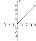
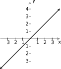
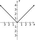
In general, the properties of integer exponents do not extend to rational exponents unless the bases involved represent non-negative real numbers or the roots involved are odd. We have the following:
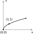
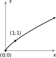
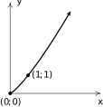
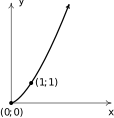
Next, we turn our attention to the graphs of for varying values of and . When is even, the domain is restricted owing to the presence of the even indexed root to . The range is likewise , a fact leave to the reader. All of the functions below are increasing on their domains, and it turns out this is always the case provided . There is, however, is a difference in how the functions are increasing - and this is the concept of concavity. As with many concepts we've encountered so far in the text, concavity is most precisely defined using Calculus terminology, but we can nevertheless get a sense of concavity geometrically. For us, a curve is concave up over an interval if it resembles a portion of a `' shape. Similarly, a curve is called concave down over an interval if resembles part of a `' shape. When , the graphs of resemble the left half of and so are concave down; when , the graphs resemble the right half of a `' and are hence described as `concave up.'
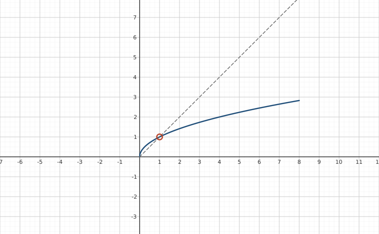
Below we graph several examples of where is odd. Here, the domain is since the index on the root here is odd. Note that when is even, the graphs appear to be symmetric about the -axis and the range looks to be . When is odd, the graphs appear to be symmetric about the origin with range . We leave verification of these facts to the reader. Note here also that for , the graphs are down for and concave up for .
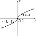
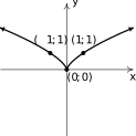
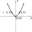
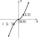
When , we have variables appear in the denominator which open the opportunities for vertical and horizontal asymptotes. Below are graphed two examples
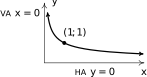
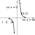
Unsurprisingly, Theorem 4.1, which, as stated, applied to root functions, generalizes to all rational powers.
The proof of Theorem 4.4 is identical to that of Theorem 4.1, and we suggest the reader work through the details. We give Theorem 4.4 a test run in the following example.
We now turn our attention to more complicated functions involving rational exponents.
Real Number Exponents
We wish now to extend the concept of `exponent' from rational to all real numbers which means we need to discuss how to interpret an irrational exponent. Once again, the notions presented here are best discussed using the language of Calculus or Analysis, but we nevertheless do what we can with the notions we have.
Consider the wildly famous irrational number . The number is defined geometrically as the ratio of the circumference of a circle to that circle's diameter.6 The reason we use the symbol `' instead of any numerical expression is that is an irrational number, and, as such, its decimal representation neither terminates nor repeats. Hence we approximate as or . No matter how many digits we write, however, what we have is a rational number approximation of .
The good news is we can approximate to any desired accuracy using rational numbers by taking enough digits, so while we'll never `reach' the exact value of with rational numbers, we can get as close as we like to using rational numbers. That being said, we assume exists on the real number line, despite the fact the list of digits to pinpoint its location is, in some sense, infinite.
We take this tack when defining the value of a number raised to an irrational exponent. Consider, for instance, . We can compute , , , and so on, so one way to define as the unique real number we obtain as the exponents `approach' .
It is with this understanding that we present the notion of a `power function,' as described in Definition 4.2: where and are nonzero real number parameters. Here the exponent is open to any (nonzero) real number. Because of how we define real number exponents, if is irrational, then to avoid having negatives under even-indexed roots as we go through the approximation process.7
In general, real number exponents inherit their properties from rational number exponents. For instance, Theorem 4.3 also holds for all real number exponents and the graphs of power functions inherit their behavior from graphs of rational exponent functions. More specifically, the graphs of functions of the form where all contain the points and . Moreover, these functions are increasing and their graphs are concave down if and concave up if .
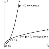
Theorem 4.4 generalizes to real number power functions, so, for instance to graph , one need only start with and shift horizontally two units to the right. (See the Exercises.)
We close this section with an application to economics. According to the US Census , Table 2, the share of money income (2014-2015) is given in the table below on the left. From these data, we can create a cumulative distribution, called the Lorenz Curve.
The number gives the percentage of the total national income earned by the bottom percent of wage earners, ranked from lowest income to highest income. Since the population here is separated into `quintiles,' each data point corresponds to of the population. So, for example, is the percentage of money income earned by the lowest of wage earners. In this case, we see . The number is the percentage of the money income earned by the bottom of wage earners - so this includes not only the money from the Second Quintile, but also the Lowest Quintile: . Likewise, is the total income share of the bottom of wage earners which includes the income from the Middle, Second, and Lowest Quintiles: .
Continuing in this manner, we get and , which is what we would expect: of the income is earned by of the population. We summarize these findings below on the right.
Exercises
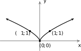
In Exercises -, use the given graphs along with Theorem 4.4 to graph the given function. Track at least two points and state the domain and range using interval notation.
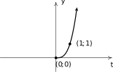
In Exercises -, find a formula for each function below in the form .
NOTE: There may be more than one solution!
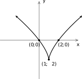
Figure 4.90 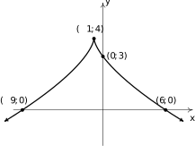
Figure 4.91
For each function in Exercises - below
Analytically:
- find the domain.
- find the axis intercepts.
- analyze the end behavior.
Graph the function with help from a graphing utility and determine:
- the range.
- the local extrema, if they exist.
- intervals of increase/decrease.
- any `unusual steepness' or `local' verticality.
- vertical asymptotes.
- horizontal / slant asymptotes.
- Construct a sign diagram for each function using the intercepts and graph.
- Comment on any observed symmetry.
For each function listed below, compute the average rate of change over the indicated interval.8 What trends do you observe? How do your answers manifest themselves graphically? Compare the results of this exercise with those of Exercise in Section 2.1 and Exercise in Section 3.1
The National Weather Service uses the following formula to calculate the wind chill:
where is the wind chill temperature in F, is the air temperature in F, and is the wind speed in miles per hour. Note that is defined only for air temperatures at or lower than F and wind speeds above miles per hour.
- Suppose the air temperature is and the wind speed is miles per hour. Find the wind chill temperature. Round your answer to two decimal places.
- Suppose the air temperature is F and the wind chill temperature is F. Find the wind speed. Round your answer to two decimal places.
As a follow-up to Exercise, suppose the air temperature is F.
- Use the formula from Exercise to find an expression for the wind chill temperature as a function of the wind speed, .
- Solve , round your answer to two decimal places, and interpret.
- Graph the function using a graphing utility and check your answer to part.
Suppose Fritzy the Fox, positioned at a point in the first quadrant, spots Chewbacca the Bunny at . Chewbacca begins to run along a fence (the positive -axis) towards his warren. Fritzy, of course, takes chase and constantly adjusts his direction so that he is always running directly at Chewbacca. If Chewbacca's speed is and Fritzy's speed is , the path Fritzy will take to intercept Chewbacca, provided is directly proportional to, but not equal to, is modeled by
- Determine the path that Fritzy will take if he runs exactly twice as fast as Chewbacca; that is, . Use your calculator to graph this path for . What is the significance of the -intercept of the graph?
- Determine the path Fritzy will take if Chewbacca runs exactly twice as fast as he does; that is, . Use a graphing utility to graph this path for . Describe the behavior of as and interpret this physically.
- With the help of your classmates, generalize parts (a) and (b) to two cases: and . We will discuss the case of in Exercise in Section 7.6.
Answers
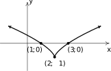
Figure 4.92 Domain: , Range: 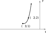
Figure 4.93 Domain: , Range: 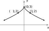
Figure 4.94 Domain: , Range: 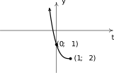
Figure 4.95 Domain: , Range: 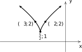
Figure 4.96 Domain: , Range: 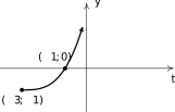
Figure 4.97 Domain: , Range: - One solution is:
- One solution is:
Domain: Intercepts: , Graph:
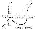
Figure 4.98 , 9 Range: Local minimum: Local maximum: (this is a cusp) Increasing: , Decreasing: Unusual steepness at
Sign Diagram:
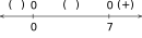
Figure 4.99 Graph:
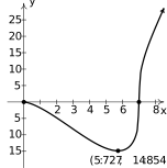
Figure 4.100 Domain: Intercepts: , Range: Local minimum: Increasing: Decreasing: Unusual steepness at Sign Diagram:

Figure 4.101 Graph:
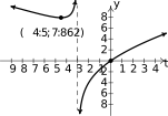
Figure 4.102 Domain: Intercept: Range: Local minimum: Increasing: , Decreasing: Vertical Asymptote: Sign Diagram:
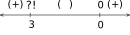
Figure 4.103 Domain: Graph:
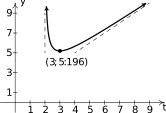
Figure 4.104 10 Range: Local minimum: Increasing: Decreasing: Vertical asymptote: Sign Diagram:

Figure 4.105 Graph:
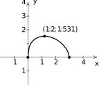
Figure 4.106 Domain: Intercepts: , Range: Increasing: Decreasing: Unusual Steepness:11 , Sign Diagram:
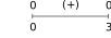
Figure 4.107 Graph:
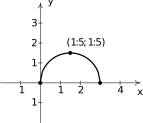
Figure 4.108 Domain: Intercepts: , Range: Increasing: Decreasing: Unusual Steepness:12 , Sign Diagram:
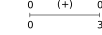
Figure 4.109 Graph:
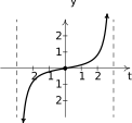
Figure 4.110 Domain: Intercepts: Range: , Vertical asymptotes: and Increasing: Sign Diagram:
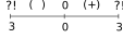
Figure 4.111 Note: is odd
Domain: Graph:
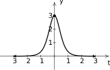
Figure 4.112 Intercept: Range: Increasing: Decreasing: Horizontal asymptote: Sign Diagram:
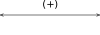
Figure 4.113 Note: is even
As in Exercise in Section 2.1 and Exercise in Section 3.1, the slopes of these curves near approach the value of the exponent on .
- F.
- miles per hour.
- . Since we are told in Exercise that wind chill is only effect for wind speeds of more than 3 miles per hour, we restrict the domain to .
- when . This means, according to the model, for the wind chill temperature to be F, the wind speed needs to be miles per hour.
The graph of is below.
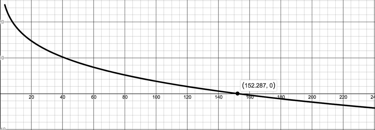
Figure 4.114
. The point is when Fritzy's path crosses Chewbacca's path - in other words, where Fritzy catches Chewbacca.
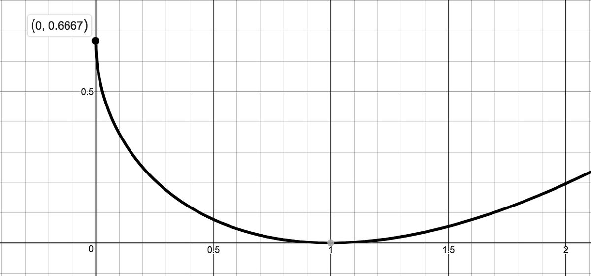
Figure 4.115 . We find as , which means, in this case, Fritzy's pursuit never ends; he never catches Chewbacca. This makes sense since Chewbacca has a head start and is running faster than Fritzy.
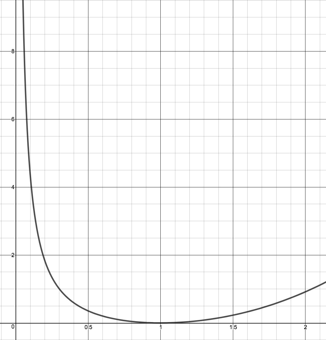
Figure 4.116
Adapted from Precalculus with Integrated Calculus, edition 4i, by Carl Stitz and Jeff Zeager (stitz-zeager.com), licensed under CC BY-NC-SA 3.0. Changes were made: reformatted as an accessible XYZ web edition. License: CC-BY-NC-SA-3.0.