
4.1 Root and Radical Functions
In Sections 1.2, 1.3 and 1.4, we studied constant, linear, absolute value,1 and quadratic functions. Constant, linear and quadratic functions were specific examples of polynomial functions, which we studied in generality in Chapter 2. Chapter 2 culminated with the Real Factorization Theorem, Theorem 2.18, which says that all polynomial functions with real coefficients can be thought of as products of linear and quadratic functions. Our next step was to enlarge our field2 of study to rational functions in Chapter 3. Being quotients of polynomials, we can ultimately view this family of functions as being built up of linear and quadratic functions as well. So in some sense, Sections 1.2, 1.3 and 1.4 along with Chapters 2 and 3 can be thought of as an exhaustive study of linear and quadratic3 functions. We now turn our attention to functions involving radicals which cannot be written in terms of linear functions. For a more detailed review of the basics of roots and radicals, we refer the reader to Sections A.2 and A.13.
Root Functions
As with polynomial functions and rational functions, we begin our study of functions involving radical with a special family of functions: the (principal) root functions.
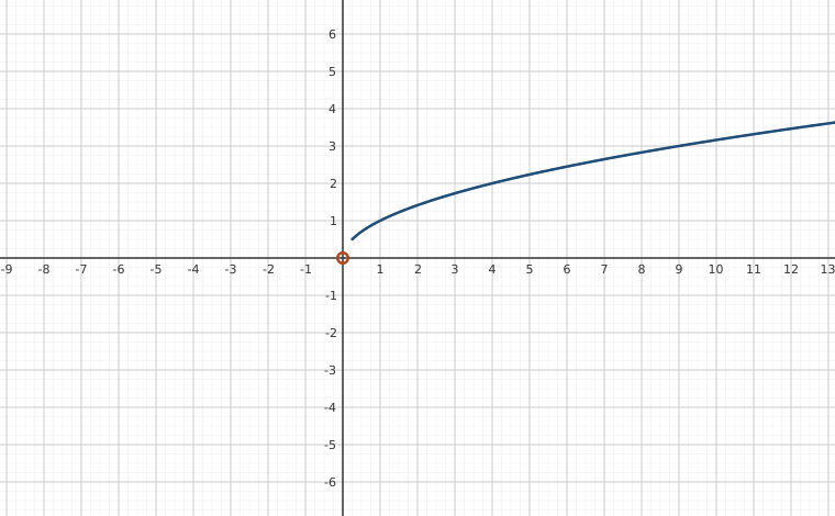
The domain restriction for even indexed roots means that, once again, we are restricting our attention to real numbers.4 We graph a few members of the root function family below, and quickly notice that, as with the monomial, and, more generally, the Laurent monomial functions, the behavior of the root functions depends primarily on whether the root is even or odd.
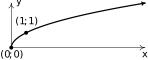
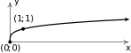
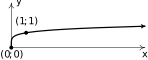
In addition to having the common domain of , the graphs of for even indices all share the points and . As increases, the functions become `steeper' near the -axis and `flatter' as . To show as , we show, more generally, the range of is . Indeed, if is a real number, then so is in the range of . Note that is increasing: that is, if , then . This property is useful in solving certain types of polynomial inequalities.5
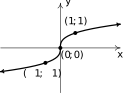
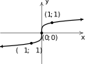
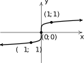
The functions for odd natural numbers also follow a predictable trend - steepening near and flattening as and . The range for these functions is since if is any real number, , so is in the range of . Like the even indexed roots, the odd indexed roots are also increasing. Moreover, these graphs appear to be symmetric about the origin. Sure enough, when is odd, so is an odd function.
At this point, you're probably expecting a theorem like Theorems 1.2, 1.3, 2.1, 3.1 - that is, a theorem which tells us how to obtain the graph of from the graph of - and you would not be wrong. Here, however, we need to add an extra parameter `' to the recipe and discuss functions of the form . The reason is that, with all of the previous function families, we were always able to factor out the coefficient of . We list some examples of this below, and invite the reader to revisit other examples in the text:
- .
- .
For a function like , this approach works fine. However, if the coefficient of is negative, for example, we get stuck the product rule for radicals doesn't extend to negative quantities when the index is even.6 Hence we add an extra parameter which means we have an extra step. We state Theorem 4.1 below.
Proof. As usual, we `build' the graph of starting with the graph of one step at a time. First, we consider the graph of . A generic point on the graph of looks like . Note that if is odd, can be any real number whereas if is even so . If we let , then and we can change (dummy) variables7 and obtain a new representation of the point: . Note that if is odd, and vary through all real numbers; if is even, and, hence, . Since a generic point on the graph of can be represented as for applicable values of , we see that we can obtain every point on the graph of by adding to each -coordinate of the graph of , establishing step 1 of the theorem.
Proceeding to (the new!) step 2, a point on the graph of has the form . If is odd, as usual, can vary through all real numbers. If is even, we require or . If , this gives . If, on the other hand, , the we have . Let and since by assumption , we have . Once again, we change dummy variables from to and describe a generic point on the graph of as . If is odd, and can vary through all real numbers. If is even and , then and, hence, ; if , then also gives . Since a generic point on the graph of can be represented as for applicable values of , we see we can obtain every point on the graph of by dividing every -coordinate on the graph of by , as per step 2 of the theorem.
The proof of steps 3 and 4 of Theorem 4.1 are identical to the proof of Theorem 2.1 (just with instead of ) so we invite the reader to work through the details on their own.
We demonstrate Theorem 4.1 in the following example.
Other Functions involving Radicals
Now that we have some practice with basic root functions, we turn our attention to more general functions involving radicals. In general, Calculus is the best tool with which to study these functions. Nevertheless, we will use what algebra we know in combination with a graphing utility to help us visualize these functions and preview concepts which are studied in greater depth in later courses. In the table below, we summarize some of the properties of radicals from elsewhere in this text (and Intermediate Algebra) we will be using in the coming examples.
We end this section with a classic application of root functions.
Exercises
In Exercises -, given the pair of functions and , sketch the graph of by starting with the graph of and using Theorem 4.1. Track at least two points and state the domain and range using interval notation.
- ,
- ,
- ,
- ,
- ,
- ,
- ,
- ,
In Exercises -, find a formula for each function below in the form .
NOTE: There may be more than one solution!
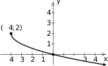
Figure 4.29 ,-intercept 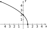
Figure 4.30 -intercept , -intercept
In Exercises -, find a formula for each function below in the form .
NOTE: There may be more than one solution!
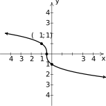
Figure 4.31 -intercept ,-intercept 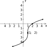
Figure 4.32 -intercept , -intercept Use the fact that the th root functions are increasing to solve the following polynomial inequalities:
For the following inequalities, remember if is even:
For each function in Exercises - below
Analytically:
- find the domain.
- find the axis intercepts.
- analyze the end behavior.
Graph the function with help from a graphing utility and determine:
- the range.
- the local extrema, if they exist.
- intervals of increase/decrease.
- any `unusual steepness' or `local' verticality.
- vertical asymptotes.
- horizontal / slant asymptotes.
- Construct a sign diagram for each function using the intercepts and graph.
- Comment on any observed symmetry.
- Rework Example 4.1.3 so that the outpost is 10 miles from Route 117 and the nearest junction box is 30 miles down the road for the post.
The volume of a right cylindrical cone depends on the radius of its base and its height and is given by the formula . The surface area of a right cylindrical cone also depends on and according to the formula . In the following problems, suppose a cone is to have a volume of 100 cubic centimeters.
- Use the formula for volume to find the height as a function of , .
- Use the formula for surface area along with your answer to to find the surface area as a function of , .
- Use your calculator to find the values of and which minimize the surface area. What is the minimum surface area? Round your answers to two decimal places.
The period of a pendulum in seconds is given by
(for small displacements) where is the length of the pendulum in meters and meters per second per second is the acceleration due to gravity. My Seth-Thomas antique schoolhouse clock needs second and I can adjust the length of the pendulum via a small dial on the bottom of the bob. At what length should I set the pendulum?
According to Einstein's Theory of Special Relativity, the observed mass of an object is a function of how fast the object is traveling. Specifically, if is the mass of the object at rest, is the speed of the object and is the speed of light, then the observed mass of the object is given by:
- Find the applied domain of the function.
- Compute and .
- Find .
- How slowly must the object be traveling so that the observed mass is no greater than 100 times its mass at rest?
- Find the inverse of .
Answers
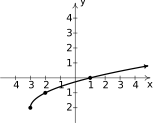
Figure 4.33 Domain: , Range: 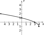
Figure 4.34 Domain: , Range: 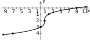
Figure 4.35 Domain: , Range: 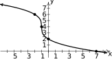
Figure 4.36 Domain: , Range: 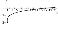
Figure 4.37 Domain: , Range: 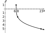
Figure 4.38 Domain: , Range: 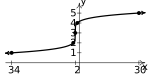
Figure 4.39 Domain: , Range: 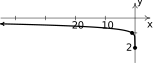
Figure 4.40 Domain: , Range: - One solution is:
- One solution is:
- One solution is:
- One solution is:
Domain: Intercepts: , Range: Local maximum: Increasing: , Decreasing: Unusual steepness20 at and Sign Diagram:

Figure 4.41 Graph:
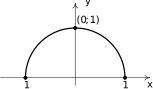
Figure 4.42 Note: is even.
Domain: Intercepts: , 21 Range: Increasing: , Decreasing: Unusual steepness22at and Sign Diagram:
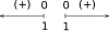
Figure 4.43 Graph:
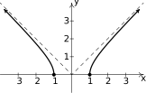
Figure 4.44 Note: is even.
Domain: Intercepts: , , Range: Local minimum Local maximum: Increasing: Decreasing: , Unusual steepness at and Sign Diagram:
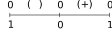
Figure 4.45 Graph:
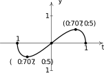
Figure 4.46 Note: is odd.
Domain: Intercepts: , Range: Increasing: , Unusual steepness at and Sign Diagram:
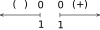
Figure 4.47 Graph:
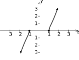
Figure 4.48 Note: is odd.
Domain: Intercept: Range: Decreasing: , Unusual steepness at Vertical asymptotes: and Horizontal asymptote: Sign Diagram:
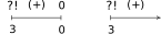
Figure 4.49 Graph:
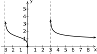
Figure 4.50 Domain: Intercept: Range: Increasing: , Vertical asymptote Horizontal asymptote Sign Diagram:
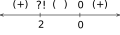
Figure 4.51 Graph:
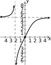
Figure 4.52 Domain: Intercepts , , Range: Local maximum Increasing: , Decreasing: Unusual steepness at and Sign Diagram:
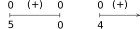
Figure 4.53 Graph:
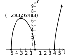
Figure 4.54 Domain: Intercepts: , , , 23 Range: Local maximum: Local minimum: Increasing: , Decreasing: Unusual steepness at and
Sign Diagram:
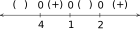
Figure 4.55 Graph:
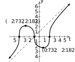
Figure 4.56 - , . The calculator gives the absolute minimum at approximately . This means to minimize the cost, approximately 18.66 miles of cable should be run along Route 117 before turning off the road and heading towards the outpost. The minimum cost to run the cable is approximately .
- , .
- ,
- The calculator gives the absolute minimum at the point . This means the radius should be (approximately) 4.07 centimeters and the height should be 5.76 centimeters to give a minimum surface area of 90.23 square centimeters.
- meters or centimeters
- , , , .
- ; as the object's velocity approaches the speed of light, mass becomes infinite.
- If the object is traveling no faster than approximately times the speed of light, then its observed mass will be no greater than .
Adapted from Precalculus with Integrated Calculus, edition 4i, by Carl Stitz and Jeff Zeager (stitz-zeager.com), licensed under CC BY-NC-SA 3.0. Changes were made: reformatted as an accessible XYZ web edition. License: CC-BY-NC-SA-3.0.