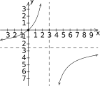
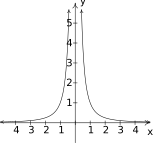
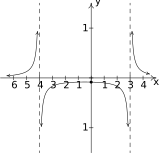
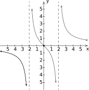
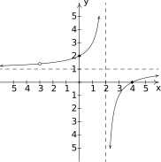
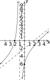
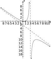
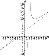
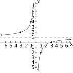
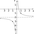
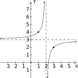
In this section, we take a closer look at graphing rational functions. In Section 4.1, we learned that the graphs of rational functions may have holes in them and could have vertical, horizontal and slant asymptotes. Theorems 4.1, 4.2 and 4.3 tell us exactly when and where these behaviors will occur, and if we combine these results with what we already know about graphing functions, we will quickly be able to generate reasonable graphs of rational functions.
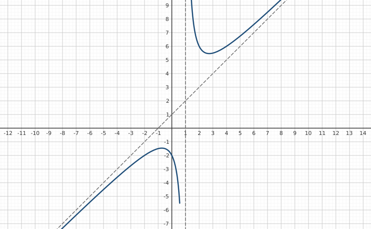
Interactive figureA slant asymptote: y = (x² + c)/(x − 1) and the line y = x + 1Drag the Constant term c slider from -4 to 6.
XYZ Graph · viewer build 5edf91b
When the numerator's degree is exactly one more than the denominator's, long division gives a linear quotient and that line is the slant asymptote. Here (x² + c)/(x − 1) = x + 1 + (1 + c)/(x − 1), so the dashed slant line y = x + 1 is the end behaviour whatever c is, and the dashed vertical line x = 1 is the vertical asymptote. The slider c changes the remainder: at c = −1 the remainder vanishes, the graph becomes the line itself with a hole at x = 1, and for other values the two branches bend away from the line near the asymptote and settle onto it far out.
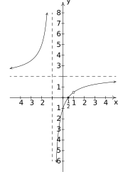
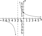
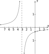
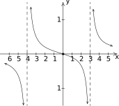
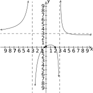
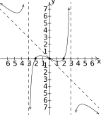
One of the standard tools we will use is the sign diagram which was first introduced in Section 2.4, and then revisited in Section 3.1. In those sections, we operated under the belief that a function couldn't change its sign without its graph crossing through the -axis. The major theorem we used to justify this belief was the Intermediate Value Theorem, Theorem 3.1. It turns out the Intermediate Value Theorem applies to all continuous functions,1 not just polynomials. Although rational functions are continuous on their domains,2 Theorem 4.1 tells us that vertical asymptotes and holes occur at the values excluded from their domains. In other words, rational functions aren't continuous at these excluded values which leaves open the possibility that the function could change sign without crossing through the -axis. Consider the graph of from Example 4.1.1, recorded below for convenience. We have added its -intercept at for the discussion that follows. Suppose we wish to construct a sign diagram for . Recall that the intervals where , or , correspond to the -values where the graph of is above the -axis; the intervals on which , or correspond to where the graph is below the -axis.
Figure 4.16Figure 4.17
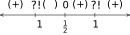
As we examine the graph of , reading from left to right, we note that from , the graph is above the -axis, so is there. At , we have a vertical asymptote, at which point the graph `jumps' across the -axis. On the interval , the graph is below the -axis, so is there. The graph crosses through the -axis at and remains above the -axis until , where we have a `hole' in the graph. Since is undefined, there is no sign here. So we have as on the interval . Continuing, we see that on , the graph of is above the -axis, so we mark there. To construct a sign diagram from this information, we not only need to denote the zero of , but also the places not in the domain of . As is our custom, we write `' above on the sign diagram to remind us that it is a zero of . We need a different notation for and , and we have chosen to use `‽' - a nonstandard symbol called the interrobang. We use this symbol to convey a sense of surprise, caution and wonderment - an appropriate attitude to take when approaching these points. The moral of the story is that when constructing sign diagrams for rational functions, we include the zeros as well as the values excluded from the domain.
Steps for Constructing a Sign Diagram for a Rational Function
Suppose is a rational function.
Place any values excluded from the domain of on the number line with an `‽' above them.
Find the zeros of and place them on the number line with the number above them.
Choose a test value in each of the intervals determined in steps 1 and 2.
Determine the sign of for each test value in step 3, and write that sign above the corresponding interval.
We now present our procedure for graphing rational functions and apply it to a few exhaustive examples. Please note that we decrease the amount of detail given in the explanations as we move through the examples. The reader should be able to fill in any details in those steps which we have abbreviated.
Steps for Graphing Rational Functions
Suppose is a rational function.
Find the domain of .
Reduce to lowest terms, if applicable.
Find the - and -intercepts of the graph of , if they exist.
Determine the location of any vertical asymptotes or holes in the graph, if they exist. Analyze the behavior of on either side of the vertical asymptotes, if applicable.
Analyze the end behavior of . Find the horizontal or slant asymptote, if one exists.
Use a sign diagram and plot additional points, as needed, to sketch the graph of .
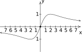
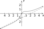
A couple of notes are in order. First, the graph of certainly seems to possess symmetry with respect to the origin. In fact, we can check to see that is an odd function. In some textbooks, checking for symmetry is part of the standard procedure for graphing rational functions; but since it happens comparatively rarely9 we'll just point it out when we see it. Also note that while is the horizontal asymptote, the graph of actually crosses the -axis at . The myth that graphs of rational functions can't cross their horizontal asymptotes is completely false,10 as we shall see again in our next example.
Our next example gives us an opportunity to more thoroughly analyze a slant asymptote.
We end this section with an example that shows it's not all pathological weirdness when it comes to rational functions and technology still has a role to play in studying their graphs at this level.
As usual, the authors offer no apologies for what may be construed as `pedantry' in this section. We feel that the detail presented in this section is necessary to obtain a firm grasp of the concepts presented here and it also serves as an introduction to the methods employed in Calculus. As we have said many times in the past, your instructor will decide how much, if any, of the kinds of details presented here are `mission critical' to your understanding of Precalculus. Without further delay, we present you with this section's Exercises.
Exercises
In Exercises -, use the six-step procedure to graph the rational function. Be sure to draw any asymptotes as dashed lines.
In Exercises -, graph the rational function by applying transformations to the graph of .
(Hint: Divide)
(Hint: Divide)
Discuss with your classmates how you would graph . What restrictions must be placed on and so that the graph is indeed a transformation of ?
In Example 3.1.1 in Section 3.1 we showed that is not a polynomial even though its formula reduced to for . However, it is a rational function similar to those studied in the section. With the help of your classmates, graph .
Let With the help of your classmates, find the - and - intercepts of the graph of . Find the intervals on which the function is increasing, the intervals on which it is decreasing and the local extrema. Find all of the asymptotes of the graph of and any holes in the graph, if they exist. Be sure to show all of your work including any polynomial or synthetic division. Sketch the graph of , using more than one picture if necessary to show all of the important features of the graph.
Example 4.2.4 showed us that the six-step procedure cannot tell us everything of importance about the graph of a rational function. Without Calculus, we need to use our graphing calculators to reveal the hidden mysteries of rational function behavior. Working with your classmates, use a graphing calculator to examine the graphs of the rational functions given in Exercises -. Compare and contrast their features. Which features can the six-step process reveal and which features cannot be detected by it?
Answers
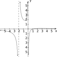
Domain: No -intercepts -intercept: Vertical asymptote: As As Horizontal asymptote: As As
Figure 4.33
Domain:
-intercept:
-intercept: Vertical asymptote: As As Horizontal asymptote: As As
Figure 4.34
Domain: No -intercepts No -intercepts Vertical asymptote: As As Horizontal asymptote: As As
Figure 4.35
Domain: No -intercepts -intercept: Vertical asymptotes: and As As As As Horizontal asymptote: As As
Figure 4.36
Domain: No -intercepts -intercept:
Hole in the graph at Vertical asymptote: As As Horizontal asymptote: As As
Figure 4.37
Domain:
-intercept:
-intercept: Vertical asymptotes: and As As As As Horizontal asymptote: As As
Figure 4.38
Domain:
-intercept:
-intercept: No vertical asymptotes No holes in the graph Horizontal asymptote: As As
Figure 4.39
Domain:
-intercept:
-intercept: Vertical asymptotes: As As As As No holes in the graph Horizontal asymptote: As As
Figure 4.40
Domain:
-intercept:
-intercept: Vertical asymptote: As As Hole at Horizontal asymptote: As As
Figure 4.41
Domain:
-intercepts: ,
-intercept: Vertical asymptotes: As As As As No holes in the graph Horizontal asymptote: As As
Figure 4.42
Domain:
-intercepts: ,
-intercept: Vertical asymptote: As As Slant asymptote: As , the graph is above As , the graph is below
Figure 4.43
Domain:
-intercepts: ,
-intercept: Vertical asymptote: As As Slant asymptote: As , the graph is above As , the graph is below
Figure 4.44
Domain:
-intercept:
-intercept: Vertical asymptote: As As Hole at Slant asymptote: As , the graph is below As , the graph is above
Figure 4.45
Domain:
-intercepts:
-intercept: Vertical asymptotes: As As As As Slant asymptote: As , the graph is above As , the graph is below
Figure 4.46
Domain:
-intercept:
-intercept: Slant asymptote: As , the graph is below As , the graph is above
Figure 4.47
Domain:
No -intercepts No -intercepts Vertical asymptotes: and As As As As Hole in the graph at Horizontal asymptote: As As
Figure 4.48
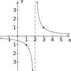
Shift the graph of to the right 2 units.
Figure 4.49
Vertically stretch the graph of by a factor of 3. Reflect the graph of about the -axis. Shift the graph of up 1 unit.
Figure 4.50
Shift the graph of down 2 units.
Figure 4.51
Shift the graph of to the right 2 units. Reflect the graph of about the -axis. Shift the graph of up 3 units.
Figure 4.52
Adapted from Precalculus, 3rd corrected edition, by Carl Stitz and Jeff Zeager (stitz-zeager.com), licensed under CC BY-NC-SA 3.0. Changes were made: reformatted as an accessible XYZ web edition. License: CC-BY-NC-SA-3.0.
These eBooks are a prerelease and are not yet certified conformant with WCAG 2.1 AA or ADA Title II. Every page is built against an automated accessibility gate, and the published editions will meet ADA Title II requirements when they release in late September 2026. If something is unusable, please tell us.