In Section 3.2, we found that we can use synthetic division to determine if a given real number is a zero of a polynomial function. This section presents results which will help us determine good candidates to test using synthetic division. There are two approaches to the topic of finding the real zeros of a polynomial. The first approach (which is gaining popularity) is to use a little bit of Mathematics followed by a good use of technology like graphing calculators. The second approach (for purists) makes good use of mathematical machinery (theorems) only. For completeness, we include the two approaches but in separate subsections.1 Both approaches benefit from the following two theorems, the first of which is due to the famous mathematician Augustin Cauchy. It gives us an interval on which all of the real zeros of a polynomial can be found.
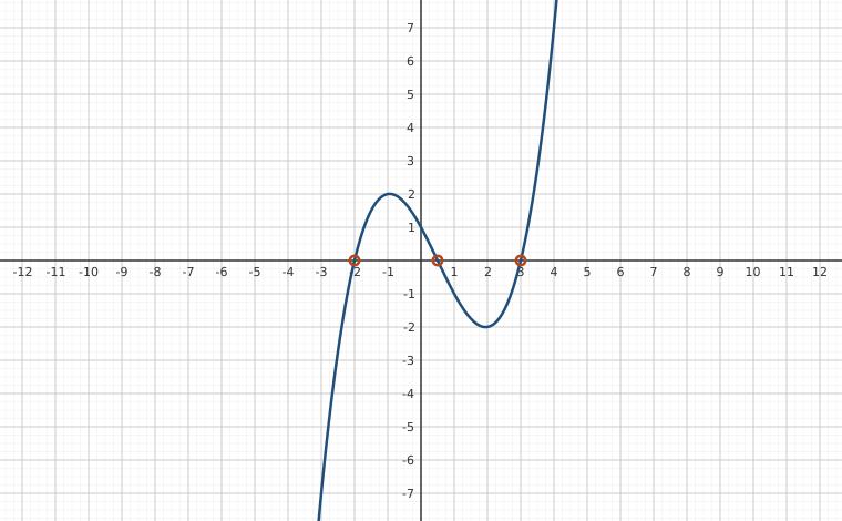
Interactive figureThree dials, three zeros: a cubic is built from its real zerosDrag the Zero r, Zero s and Zero u sliders.
XYZ Graph · viewer build 5edf91b
The curve is p(x) = (x − r)(x − s)(x − u)/3, so its real zeros are the three slider values and nothing else; the marked points on the x-axis are exactly those zeros. Slide any dial and its intercept slides with it while the curve bends to keep passing through all three. Push two dials together and the curve stops crossing there and merely touches the axis, a zero of multiplicity two; pull them apart and the crossing returns. The picture is the bound-and-test strategy of this section run backwards: knowing where the zeros are tells you the shape, and the shape tells you where to test.
The proof of this fact is not easily explained within the confines of this text. This paper contains the result and gives references to its proof. Like many of the results in this section, Cauchy's Bound is best understood with an example.
Whereas the previous result tells us where we can find the real zeros of a polynomial, the next theorem gives us a list of possible real zeros.
The Rational Zeros Theorem gives us a list of numbers to try in our synthetic division and that is a lot nicer than simply guessing. If none of the numbers in the list are zeros, then either the polynomial has no real zeros at all, or all of the real zeros are irrational numbers. To see why the Rational Zeros Theorem works, suppose is a zero of and in lowest terms. This means and have no common factors. Since , we have
Multiplying both sides of this equation by , we clear the denominators to get
Rearranging this equation, we get
Now, the left hand side is an integer multiple of , and the right hand side is an integer multiple of . (Can you see why?) This means is both a multiple of and a multiple of . Since and have no common factors, must be a multiple of . If we rearrange the equation
as
we can play the same game and conclude is a multiple of , and we have the result.
Our discussion now diverges between those who wish to use technology and those who do not.
For Those Wishing to use a Graphing Calculator
At this stage, we know not only the interval in which all of the zeros of are located, but we also know some potential candidates. We can now use our calculator to help us determine all of the real zeros of , as illustrated in the next example.
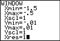
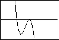
It is interesting to note that we could greatly improve on the graph of in the previous example given to us by the calculator. For instance, from our determination of the zeros of and their multiplicities, we know the graph crosses at then turns back upwards to touch the axis at . This tells us that, despite what the calculator showed us the first time, there is a relative maximum occurring at and not a `flattened crossing' as we originally believed. After resizing the window, we see not only the relative maximum but also a relative minimum2 just to the left of which shows us, once again, that Mathematics enhances the technology, instead of vice-versa.
Figure 3.49Figure 3.50
Our next example shows how even a mild-mannered polynomial can cause problems.
The technique used to factor in Example 3.3.4 is called
-substitution. We shall see more of this technique in Section 5.3. In general, substitution can help us identify a `quadratic in disguise' provided that there are exactly three terms and the exponent of the first term is exactly twice that of the second. It is entirely possible that a polynomial has no real roots at all, or worse, it has real roots but none of the techniques discussed in this section can help us find them exactly. In the latter case, we are forced to approximate, which in this subsection means we use the `Zero' command on the graphing calculator.
For Those Wishing NOT to use a Graphing Calculator
Suppose we wish to find the zeros of
without using the calculator. In this subsection, we present some more advanced mathematical tools (theorems) to help us. Our first result is due to René Descartes.
A few remarks are in order. First, to use Descartes' Rule of Signs, we need to understand what is meant by a `variation in sign' of a polynomial function. Consider . If we focus on only the signs of the coefficients, we start with a , followed by another , then switch to , and stay for the remaining two coefficients. Since the signs of the coefficients switched once as we read from left to right, we say that has one variation in sign. When we speak of the variations in sign of a polynomial function we assume the formula for is written with descending powers of , as in Definition 3.1, and concern ourselves only with the nonzero coefficients. Second, unlike the Rational Zeros Theorem, Descartes' Rule of Signs gives us an estimate to the number of positive and negative real zeros, not the actual value of the zeros. Lastly, Descartes' Rule of Signs counts multiplicities. This means that, for example, if one of the zeros has multiplicity , Descsartes' Rule of Signs would count this as two zeros. Lastly, note that the number of positive or negative real zeros always starts with the number of sign changes and decreases by an even number. For example, if has sign changes, then, counting multplicities, has either , , or positive real zero. This implies that the graph of crosses the positive -axis at least once. If results in sign changes, then, counting multiplicities, has , or negative real zeros; hence, the graph of may not cross the negative -axis at all. The proof of Descartes' Rule of Signs is a bit technical, and can be found here.
Cauchy's Bound gives us a general bound on the zeros of a polynomial function. Our next result helps us determine bounds on the real zeros of a polynomial as we synthetically divide which are often sharper3 bounds than Cauchy's Bound.
The Upper and Lower Bounds Theorem works because of Theorem 3.4. For the upper bound part of the theorem, suppose is divided into and the resulting line in the division tableau contains, for example, all nonnegative numbers. This means , where the coefficients of the quotient polynomial and the remainder are nonnegative. (Note that the leading coefficient of is the same as so is not the zero polynomial.) If , then , where and are both positive and . Hence which shows cannot be a zero of . Thus no real number can be a zero of , as required. A similar argument proves if all of the numbers in the final line of the synthetic division tableau are non-positive. To prove the lower bound part of the theorem, we note that a lower bound for the negative real zeros of is an upper bound for the positive real zeros of . Applying the upper bound portion to gives the result. (Do you see where the alternating signs come in?) With the additional mathematical machinery of Descartes' Rule of Signs and the Upper and Lower Bounds Theorem, we can find the real zeros of without the use of a graphing calculator.
You can see why the `no calculator' approach is not very popular these days. It requires more computation and more theorems than the alternative.4 In general, no matter how many theorems you throw at a polynomial, it may well be impossible5 to find their zeros exactly. The polynomial is one such beast.6 According to Descartes' Rule of Signs, has exactly one positive real zero, and it could have two negative real zeros, or none at all. The Rational Zeros Test gives us as rational zeros to try but neither of these work since . If we try the substitution technique we used in Example 3.3.4, we find has three terms, but the exponent on the isn't exactly twice the exponent on . How could we go about approximating the positive zero without resorting to the `Zero' command of a graphing calculator? We use the Bisection Method. The first step in the Bisection Method is to find an interval on which changes sign. We know and we find . By the Intermediate Value Theorem, we know that the zero of lies in the interval . Next, we `bisect' this interval and find the midpoint is . We have that . This means that our zero is between and , since changes sign on this interval. Now, we `bisect' the interval and find , so now we have the zero between and . Bisecting , we find , which means the zero of is between and . We continue in this fashion until we have `sandwiched' the zero between two numbers which differ by no more than a desired accuracy. You can think of the Bisection Method as reversing the sign diagram process: instead of finding the zeros and checking the sign of using test values, we are using test values to determine where the signs switch to find the zeros. It is a slow and tedious, yet fool-proof, method for approximating a real zero.
Our next example reminds us of the role finding zeros plays in solving equations and inequalities.
Our last example revisits an application from page in the Exercises of Section 3.1.
Exercises
In Exercises -, for the given polynomial:
Use Cauchy's Bound to find an interval containing all of the real zeros.
Use the Rational Zeros Theorem to make a list of possible rational zeros.
Use Descartes' Rule of Signs to list the possible number of positive and negative real zeros, counting multiplicities.
In Exercises -, find the real zeros of the polynomial using the techniques specified by your instructor. State the multiplicity of each real zero.
In Exercises -, use your calculator,8 to help you find the real zeros of the polynomial. State the multiplicity of each real zero.
Find the real zeros of by first finding a polynomial with integer coefficients such that for some integer . (Recall that the Rational Zeros Theorem required the polynomial in question to have integer coefficients.) Show that and have the same real zeros.
In Exercises -, find the real solutions of the polynomial equation. (See Example 3.3.7.)
In Exercises -, solve the polynomial inequality and state your answer using interval notation.
In Example 3.1.3 in Section 3.1, a box with no top is constructed from a inch
inch piece of cardboard by cutting out congruent squares from each corner of the cardboard and then folding the resulting tabs. We determined the volume of that box (in cubic inches) is given by , where denotes the length of the side of the square which is removed from each corner (in inches), . Solve the inequality analytically and interpret your answer in the context of that example.
From Exercise in Section 3.1, , for models the cost, in dollars, to produce PortaBoy game systems. If the production budget is , find the number of game systems which can be produced and still remain under budget.
Let . With the help of your classmates, find the - and - intercepts of the graph of . Find the intervals on which the function is increasing, the intervals on which it is decreasing and the local extrema. Sketch the graph of , using more than one picture if necessary to show all of the important features of the graph.
With the help of your classmates, create a list of five polynomials with different degrees whose real zeros cannot be found using any of the techniques in this section.
Answers
For
All of the real zeros lie in the interval
Possible rational zeros are , , ,
There are 2 or 0 positive real zeros; there is 1 negative real zero
For
All of the real zeros lie in the interval
Possible rational zeros are , , , , ,
There is 1 positive real zero; there are 3 or 1 negative real zeros
For
All of the real zeros lie in the interval
Possible rational zeros are , , , , ,
There are 2 or 0 positive real zeros; there are 2 or 0 negative real zeros
For
All of the real zeros lie in the interval
Possible rational zeros are , , ,
There are 2 or 0 positive real zeros; there is 1 negative real zero
For
All of the real zeros lie in the interval
Possible rational zeros are ,
There are 3 or 1 positive real zeros; there are no negative real zeros
For
All of the real zeros lie in the interval
Possible rational zeros are , , , , , , ,
There are 3 or 1 positive real zeros; there are no negative real zeros
For
All of the real zeros lie in the interval
Possible rational zeros are , , , , , , ,
There are 2 or 0 positive real zeros; there is 1 negative real zero
For
All of the real zeros lie in the interval
Possible rational zeros are , , , , , , , ,
There are 2 or 0 positive real zeros; there are 2 or 0 negative real zeros
For
All of the real zeros lie in the interval
Possible rational zeros are , , , , , , ,
There is 1 positive real zero; there are 2 or 0 negative real zeros
For
All of the real zeros lie in the interval
Possible rational zeros are , , ,
There are 2 or 0 positive real zeros; there are 2 or 0 negative real zeros
, , (each has mult. 1)
(mult. 3), (mult. 1)
(mult. 2), (mult. 1), (mult. 1)
(mult. 1), (mult. 2)
(mult. 1)
, , (each has mult. 1)
, (each has mult. 1)
(mult. 2), (mult. 2)
, (each has mult. 1)
, , (each mult. 1)
, (each has mult. 1)
(mult. 2), (each has mult. 1)
(each has mult. 1)
, (each has mult. 1)
(each has mult. 1)
, (each has mult. 1)
, (each has mult. 1)
, (each has mult. 1)
, (each has mult. 1)
, (each has mult. 1)
(mult. 3), (mult. 2)
(mult. 2), (mult. 3)
, , , (each has mult. 1)
We choose . Clearly if and only if so they have the same real zeros. In this case, and are the real zeros of both and .
on . Only the portion lies in the applied domain, however. In the context of the problem, this says for the volume of the box to be at least 80 cubic inches, the square removed from each corner needs to have a side length of at least 1 inch, but no more than inches.
on (approximately) . The portion of this which lies in the applied domain is . Since represents the number of game systems, we check and , so to remain within the production budget, anywhere between and game systems can be produced.
Adapted from Precalculus, 3rd corrected edition, by Carl Stitz and Jeff Zeager (stitz-zeager.com), licensed under CC BY-NC-SA 3.0. Changes were made: reformatted as an accessible XYZ web edition. License: CC-BY-NC-SA-3.0.
These eBooks are a prerelease and are not yet certified conformant with WCAG 2.1 AA or ADA Title II. Every page is built against an automated accessibility gate, and the published editions will meet ADA Title II requirements when they release in late September 2026. If something is unusable, please tell us.