9.4 Model Construction

In practice, we either don't know what the optimum model we need is, or the needs of the model change as we obtain more data.

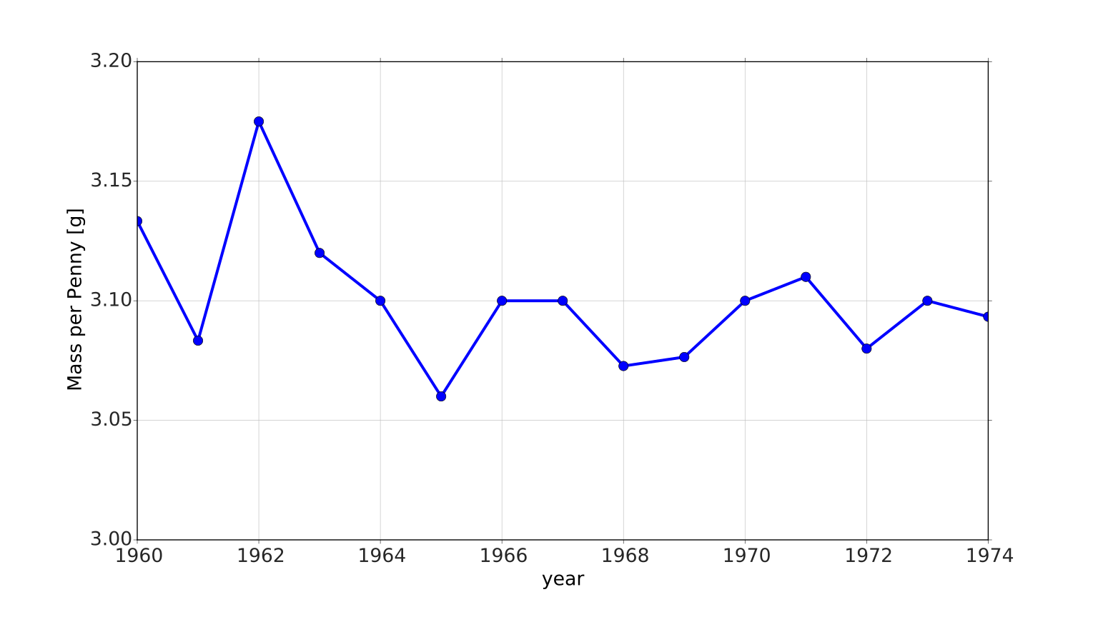
We start with the data in Table 9.4 for the mass of pennies of various years (shown graphically in Figure 9.3):

**Table 9.4.** Mass of Pennies from 1960 to 1974.
Year	Mass [g]
1960	3.133
1961	3.083
1962	3.175
1963	3.120
1964	3.100
1965	3.060
1966	3.100
1967	3.100
1968	3.073
1969	3.076
1970	3.100
1971	3.110
1972	3.080
1973	3.100
1974	3.093

Scatter of the mass of US pennies for each year from 1960 to 1974: values wander between roughly 3.06 and 3.18 grams around a typical value near 3.10 grams, with no trend over time. — **Figure 9.3.** Mass of Pennies from 1960 to 1974.

We are going to ignore the measurement uncertainties in these individual measurements, because they are quite small.

Try it in XYZ Crunch

Plot the pennies before you model them

The section's own lesson is 'always look at your data graphically' - so start with the scatter of mass against year, where the two levels are impossible to miss. Then run 1-Var Stats three ways and watch what the single-true-value model does: the 1960-74 pennies give mean 3.100 with sample deviation 0.0278, the 1989-2003 pennies give 2.507 with 0.0102, but pooling all thirty gives 2.804 with 0.3024 - a deviation eleven times either group's, which is the whole reason the model has to change.

Example 1 Mass of the Penny, Model 1 - One True Value

If we assume a model that states that there is a “true” value and the variation from this “true” value caused by some unknown process, but with known magnitude, $σ$ ,

$\begin{matrix} d a t a = true value + Normal(mean=0,known σ) \end{matrix}$

or equivalently

$d a t a equals Normal(mean= true value,known σ )$

we can get the best estimate and uncertainty in that estimate from the following procedure, Using the normal approximation to the Student-T distribution (Section 7.4):

$\begin{matrix} \hat{μ} = \bar{x} \pm k \cdot S / \sqrt{N} \end{matrix}$

where the symbols in this equation are

the number of data points, $N$ .
the best estimate for the true value, $\hat{μ}$ , is given by the sample mean, $\bar{x}$ :
$\begin{matrix} \bar{x} = = \frac{x_{1} + x_{2} + \dots + x_{N}}{N} \\ = \frac{3.133 g + 3.083 g + \dots + 3.093 g}{15} \\ = 3.100 g \end{matrix}$
The uncertainty is directly related to the sample standard deviation, $S$ :
$\begin{matrix} S = \sqrt{\frac{(x_{1} - \bar{x})^{2} + (x_{2} - \bar{x})^{2} + \dots + (x_{N} - \bar{x})^{2}}{N - 1}} \\ = \sqrt{\frac{(3.133 g - 3.100 g)^{2} + (3.083 - 3.100 g)^{2} + \dots + (3.093 - 3.100 g)^{2}}{14}} \\ = 0.0278 g \end{matrix}$
The scale factor, $k$ , adjusts for the small number of data points - there is more uncertainty in our estimate when there are fewer data points:
$\begin{matrix} k = 1 + \frac{20}{N^{2}} \\ = 1 + \frac{20}{15^{2}} \\ = 1.0889 \end{matrix}$

Finally, we have the best estimate and uncertainty for the pennies in this dataset:

$\begin{matrix} \hat{μ} = \bar{x} \pm k \cdot S / \sqrt{N} \\ = 3.100 g \pm 1.0889 \cdot 0.0278 g / \sqrt{15} \\ = 3.100 g \pm 0.0078 g \end{matrix}$

or, as a 99% credible range (3 times the uncertainty written above), we have, (see also Figure 9.4)

$\begin{matrix} 99% CI for μ = 3.100 g \pm 3 \times 0.0078 g \\ = [3.077 g, 3.124 g] \end{matrix}$

Figure 9.4. Mass of Pennies from 1960 to 1974, with best estimates and 99% CI (i.e.

3 σ

) uncertainty.

Example 2 Mass of the Penny, Model 1 - One True Value with More Data

Now we collect the additional data with more recent pennies shown in Table 9.5. We can follow the same procedure, assuming our original model of one “true” value, to get the best estimate and uncertainty for this model, combining the two data sets.

**Table 9.5.** Mass of Pennies from 1989 to 2003.
Year	Mass [g]
1989	2.516
1990	2.500
1991	2.500
1992	2.500
1993	2.503
1994	2.500
1995	2.497
1996	2.500
1997	2.494
1998	2.512
1999	2.521
2000	2.499
2001	2.523
2002	2.518
2003	2.520

$\begin{matrix} \hat{μ} = \bar{x} \pm k \cdot S / \sqrt{N} \end{matrix}$

where the symbols in this equation are

the number of data points, $N equals 30$ .
the best estimate for the true value, $\hat{μ}$ , is given by the sample mean, $\bar{x}$ :
$\begin{matrix} \bar{x} = \frac{3.133 g + 3.083 g + \dots + 2.520 g}{30} \\ = 2.804 g \end{matrix}$
The sample standard deviation, $S$ :
$\begin{matrix} S = \sqrt{\frac{(3.133 g - 2.804 g)^{2} + (3.083 - 2.804 g)^{2} + \dots + (2.520 - 2.804 g)^{2}}{29}} \\ = 0.3024 g \end{matrix}$
The scale factor, $k$ , adjusting for the small number of data points:
$\begin{matrix} k = 1 + \frac{20}{30^{2}} \\ = 1.0222 \end{matrix}$

Finally, we have the best estimate and uncertainty for the pennies in this full dataset:

$\begin{matrix} \hat{μ} = \bar{x} \pm k \cdot S / \sqrt{N} \\ = 2.804 g \pm 1.0222 \cdot 0.3024 g / \sqrt{30} \\ = 2.804 g \pm 0.0564 g \end{matrix}$

or, as a 99% credible range (3 times the uncertainty written above), we have,

$\begin{matrix} 99% CI for μ = 2.804 g \pm 3 \times 0.0564 g \\ = [2.634 g, 2.973 g] \end{matrix}$

There are several things one should notice:

The scale factor, $k$ , is less for 30 data points than it is for 15 data points. This is because the adjustment for small number of data points gets less relevant as we obtain more data. This is what we expect.
Despite there being twice as much data, our uncertainty increased. This is unusual, if our model is correct - more data should sharpen the estimates. Although it is possible that adding more data increased the system variability somehow, it is more likely that some assumption of our model is incorrect. This becomes obvious when we look at the result graphically, shown in Figure 9.5.

Figure 9.5. Mass of Pennies from 1960 to 2003, with best estimates and 99% CI (i.e.

3 σ

) uncertainty.

This should highlight a few things:

Always look at your data graphically. What you might miss looking at a table of numbers, you'll catch with a picture.
Assume your model is wrong, and outline other possible models ahead of time and explore them. The most obvious improvement in this problem is to notice that we are dealing with two separate “true” values, possibly caused by a change in the manufacturing materials.

Overlapping Intervals

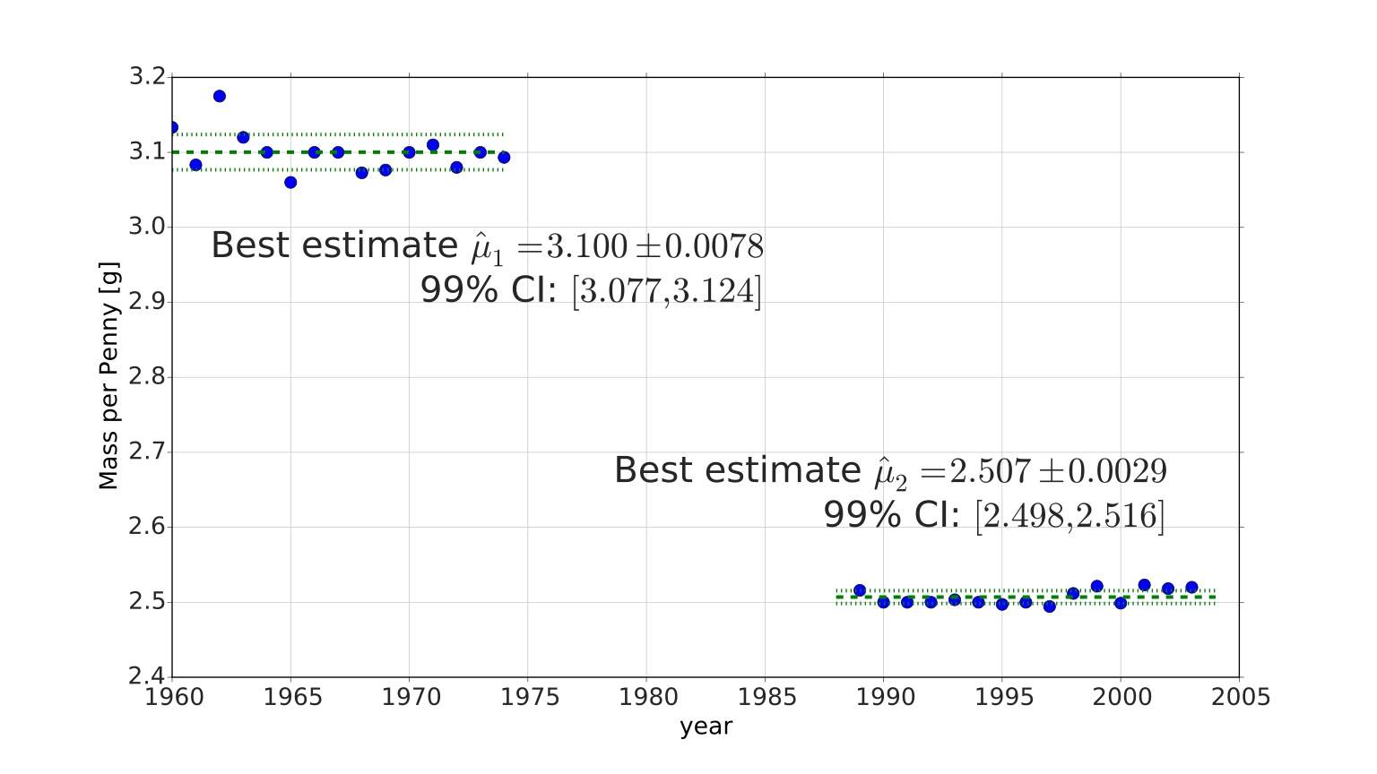
The first is the easiest to do mathematically, and yields a nice picture: obtain the best estimates for $μ sub 1$ and $μ sub 2$ , and see if their 99% credible intervals overlap. From this analysis (identical to the previous examples, however we leave the details of the calculation to the student), we get (see Figure 9.6):

Best estimate for $μ sub 1$
$μ hat sub 1 equals 3.100 ± 0.0078$
with 99% CI: [3.077,3.124].
Best estimate for $μ sub 2$
$μ hat sub 2 equals 2.507 ± 0.0029$
with 99% CI: [2.498,2.516]

where the 99% credible intervals (CI) clearly do not overlap, thus there is a statistically significant difference between them.

Penny masses from 1960 to 2003 fitted with two true values: separate dashed best-estimate lines with narrow 99% bands at about 3.10 grams (before 1975) and 2.50 grams (after 1989). The two credible intervals clearly do not overlap. — **Figure 9.6.** Mass of Pennies from 1960 to 2003, with best estimates for the two true values and their 99% CI (i.e. $3 σ$ ) uncertainty plotted. There is clearly no overlap in their credible intervals, thus there is a statistically significant difference between them.

Is the Difference Zero?

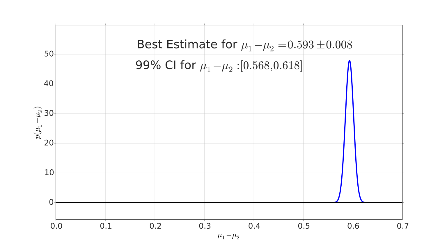
The proper way is to estimate the quantity $μ sub 1 minus μ sub 2$ and test to see if it is greater than zero, as shown in Section 7.2 on page 144. The estimate of this quantity, which we'll call $δ_{12} = μ_{1} - μ_{2}$ is related to the means and uncertainties of two data sets

$\begin{matrix} {\hat{δ}}_{12} = {\bar{x}}_{1} - {\bar{x}}_{2} \pm σ_{12} \\ σ_{12} = \sqrt{σ_{1}^{2} + σ_{2}^{2}} \\ σ_{1} = k_{1} S_{1} / \sqrt{N_{1}} (uncertainty from data set 1) \\ σ_{2} = k_{2} S_{2} / \sqrt{N_{2}} (uncertainty from data set 2) \end{matrix}$

where the sample standard deviations, $S sub 1$ and $S sub 2$ , and the scale factors, $k sub 1$ and $k sub 2$ were calculated earlier. This leads to, for this data set,

$δ hat sub 12 equals 0.593 g ± 0.008 g$

with the 99% credible interval $open bracket 0.568 g, 0.618 g close bracket$ , the distribution shown in Figure 9.7. Again, the estimated quantities are clearly different statistically: the value of zero is well outside of the 99% credible interval for $δ sub 12$ .

Posterior distribution of the difference between the pre- and post-1975 penny masses, μ1-μ2: a bell curve centered near 0.6 grams whose 99% interval excludes zero, so the mass change is statistically significant. — **Figure 9.7.** Difference in the estimated values of the pre- and post 1975 pennies, $μ sub 1 minus μ sub 2$ . The value zero is clearly outside of the 99% interval of the difference, thus there is a statistically significant difference between the two values $μ sub 1$ and $μ sub 2$ .

Adapted from Statistical Inference for Everyone, by Brian Blais (Bryant University), licensed under CC BY-SA 4.0 (dual-licensed under the GNU FDL 1.2 or later; this adaptation uses the CC BY-SA grant). Changes were made; this adaptation is distributed under the same license. License: CC-BY-SA-4.0.