
8.5 Computer Examples
from sie import *data=load_data('data/iris.csv')x_sertosa=data[data['class']=='Iris-setosa']['petal length [cm]']x=x_sertosa
mu=sample_mean(x)
N=len(x)
sigma=sample_deviation(x)/sqrt(N)
t_sertosa=tdist(N,mu,sigma)
print "total number of data points:",N
print "best estimate:",mu
print "uncertainty:",sigmaShow expected output
total number of data points: 50
best estimate: 1.464
uncertainty: 0.0245381834898new_length=1.7distplot(t_sertosa,label='petal length',xlim=[1.37,1.8],
quartiles=[.01,0.05,.5,.95,.99],
)
ax=gca()
ax.axvline(1.7,color='r')
savefig('../../figs/z_test_iris.pdf')Show expected output
<matplotlib.figure.Figure at 0x10f9d2710>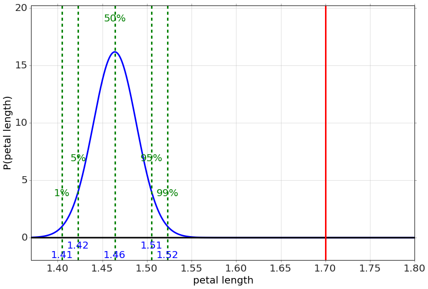
Adapted from Statistical Inference for Everyone, by Brian Blais (Bryant University), licensed under CC BY-SA 4.0 (dual-licensed under the GNU FDL 1.2 or later; this adaptation uses the CC BY-SA grant). Changes were made; this adaptation is distributed under the same license. License: CC-BY-SA-4.0.