4.2 The High/Low Deck Game

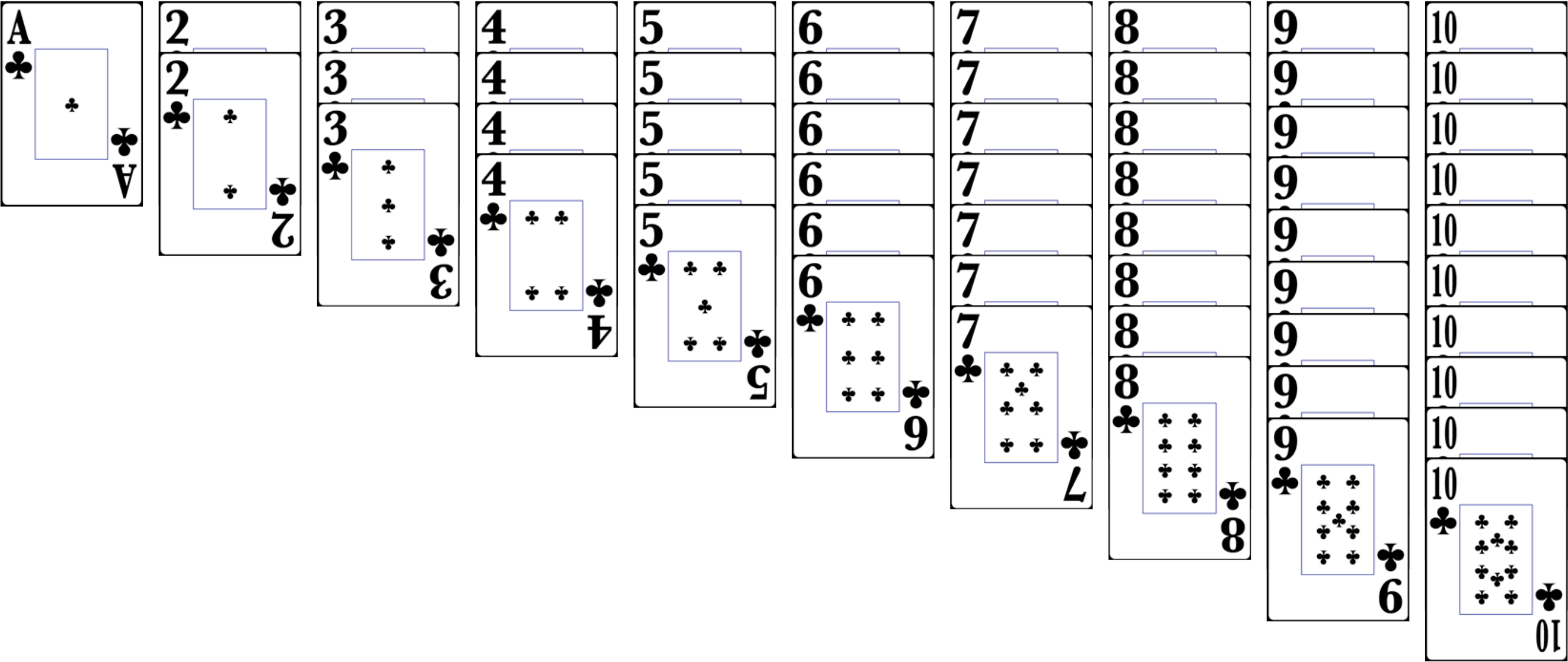
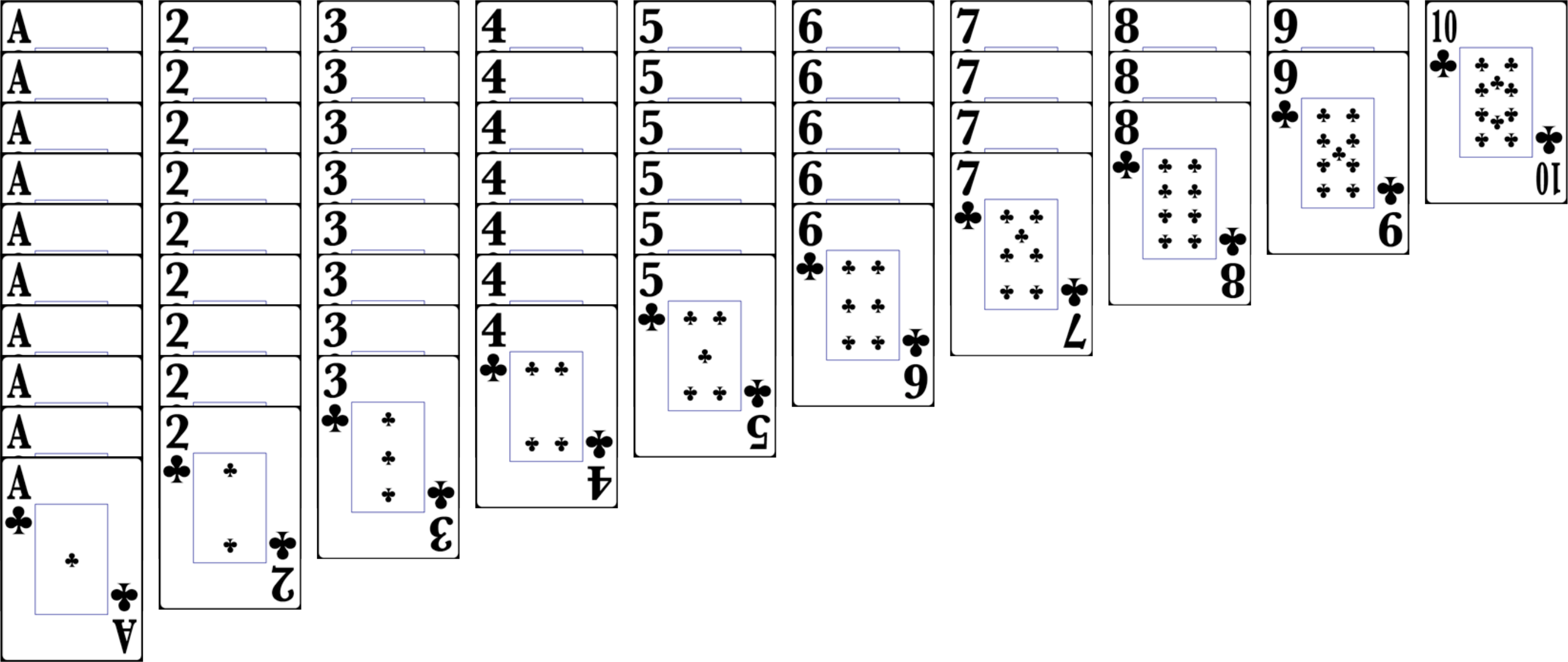
In this example we use a simple card game as a platform for discussing model comparison in general. We start with two atypical decks of cards called the High Deck and the Low Deck (Figures 4.1 on page 96 and 4.2 on page 96 respectively). The game goes as follows.

The 55-card High Deck laid out in ten columns of clubs: one Ace, two 2s, three 3s, four 4s, five 5s, six 6s, seven 7s, eight 8s, nine 9s and ten 10s — the higher the value, the more copies it has. — **Figure 4.1.** High Deck - 55 Cards with ten 10's, nine 9's, etc... down to one Ace. Aces are equivalent to the value 1.

The 55-card Low Deck laid out in ten columns of clubs: ten Aces, nine 2s, eight 3s, seven 4s, six 5s, five 6s, four 7s, three 8s, two 9s and one 10 — the lower the value, the more copies it has. — **Figure 4.2.** Low Deck - 55 Cards with ten Aces, nine 2's, etc... up to one 10. Aces are equivalent to the value 1.

What does our intuition say?

We start by exploring our intuitions, before we do anything mathematically. Thus, we are in a position to check to see if the math is reasonable before we use the same math in areas where our intuition is not as strong. Imagine we draw only one card, and it is a 9. Intuition suggests that this constitutes reasonably strong evidence toward the belief that we're holding the High Deck. If we then (as the procedure states) place the 9 back in the deck, reshuffle and then draw a 7 we can be more strongly convinced that we are holding the High Deck. Repeating the reshuffle, and then drawing a 3 would make us a little less confident in this conclusion, but still quite certain. In this way we can sense how drawing different cards pushes our belief around, depending on how often that card comes up in the different decks.

Before the data - the prior

Before we take any data, we need to quantify our state of knowledge concerning all of the models that we are considering. In this case it is quite simple, because there are two models (High Deck and Low Deck), and we have been given no information about whether either is more common. With no such information, it is equivalent to a coin flip - we assign equal probabilities to both models before we see data, also known as the prior probabilities.

$\begin{matrix} P (H) = 0.5 \\ P (L) = 0.5 \end{matrix}$

Surely this assessment will change after we see data, but that is the rest of the problem.

The “easy” question - the likelihood

Although our ultimate goal is to infer the type of deck from the cards that we draw from it, we can start looking at an easier part of this question which serves as a first step toward the more challenging, and interesting goal. That question is the following,

Example 1 What is the probability of drawing a 9, given that we know that we're holding the High Deck?

Show solution

This related question is written

$P open parenthesis d a t a equals 9 vertical bar H close parenthesis$

where $d a t a equals 9$ means that we have observed (i.e. drawn) one 9. This question is “easy” in the sense that it is simply related to the properties of the High Deck: the number of 9's and total number of cards. If you know that you have the high deck, then you know there are nine 9's in that deck out of 55 cards, and thus we have the probability of drawing one 9, given that we are holding the High Deck, is

$\begin{matrix} P (d a t a = 9 | H) = \frac{9}{55} \end{matrix}$

We give this the name likelihood, and is simply the probability that the data could be the result of a known model. It is also the first part of the top of Bayes' Rule, Equation 1.14 on page 47.

Applying the Bayes' recipe

Here we introduce for the first time a recipe we will follow for all model comparison examples.

Now that we have our intuition, and we have the likelihoods, we can address the math. The two models are:

$\begin{matrix} H \equiv ``We're holding the High Deck'' \\ L \equiv ``We're holding the Low Deck'' \end{matrix}$

and the initial data is

$d a t a ≡ ``We've drawn one card, and it is a 9''$

According to Equation 4.1 on page 95 we are looking for the two probabilities:

$\begin{matrix} P (H | d a t a = 9) \\ P (L | d a t a = 9) \end{matrix}$

which are related to the prior and the likelihood via Bayes' Rule (Equation 1.14):

$\begin{matrix} P (H | d a t a = 9) = \frac{P (d a t a = 9 | H) P (H)}{P (d a t a = 9)} \\ P (L | d a t a = 9) = \frac{P (d a t a = 9 | L) P (L)}{P (d a t a = 9)} \end{matrix}$

To calculate actual numbers, we apply the Bayes' Recipe to this problem,

Specify the prior probabilities for the models being considered
$\begin{matrix} P (H) = 0.5 \\ P (L) = 0.5 \end{matrix}$
Write the top of Bayes' Rule for all models being considered
$\begin{matrix} P (H | d a t a = 9) \sim P (d a t a = 9 | H) P (H) \\ P (L | d a t a = 9) \sim P (d a t a = 9 | L) P (L) \end{matrix}$
where we are using the symbol $∼$ to denote proportionality or related to. Essentially, by calculating the top of Bayes' Rule first, the numbers are not equal to the final (i.e. posterior) probabilities but must be rescaled to make sure that they add up to 1. This is done in the final step. Up until that rescaling, we use the symbol $∼$ and think of it as related to.
Put in the likelihood and prior values
$\begin{matrix} P (H | d a t a = 9) \sim \frac{9}{55} \times 0.5 = 0.082 \\ P (L | d a t a = 9) \sim \frac{2}{55} \times 0.5 = 0.018 \end{matrix}$
Add these values for all models
$\begin{matrix} K = 0.082 + 0.018 = 0.1 \end{matrix}$
Divide each of the values by this sum, $K$ , to get the final probabilities
$\begin{matrix} P (H | d a t a) = 0.082 / 0.1 = 0.82 \\ P (L | d a t a) = 0.018 / 0.1 = 0.18 \end{matrix}$

From which we can conclude that drawing a 9 does indeed constitute reasonably strong evidence toward the belief that we're holding the High Deck - the probability of us holding the High Deck, given the data, is 0.82.

Drawing the next card

So, when we draw a 7 next (after reshuffling), our intuition suggests that we'd be more confident that we're holding the High Deck. Repeating our recipe we have

The two models are:

$\begin{matrix} H \equiv ``We're holding the High Deck'' \\ L \equiv ``We're holding the Low Deck'' \end{matrix}$

and data is

$d a t a ≡ open brace ``We've drawn one card, and it is a 9, replaced and reshuffled, and then drawn a 7''$

According to Equation 4.1 we are looking for the two probabilities:

$\begin{matrix} P (H | d a t a = 9 then a 7) \\ P (L | d a t a = 9 then a 7) \end{matrix}$

which are related to the prior and the likelihood via Bayes' Rule (Equation 1.14):

$\begin{matrix} P (H | d a t a = 9 then a 7) = \frac{P (d a t a = 9 then a 7 | H) P (H)}{P (d a t a = 9 then a 7)} \\ P (L | d a t a = 9 then a 7) = \frac{P (d a t a = 9 then a 7 | L) P (L)}{P (d a t a = 9 then a 7)} \end{matrix}$

To calculate actual numbers, we apply the Bayes' recipe to this problem,

Specify the prior probabilities for the models being considered
$\begin{matrix} P (H) = 0.5 \\ P (L) = 0.5 \end{matrix}$
Write the top of Bayes' Rule for all models being considered
$\begin{matrix} P (H | d a t a = 9 then a 7) \sim P (d a t a = 9 then a 7 | H) P (H) \\ P (L | d a t a = 9 then a 7) \sim P (d a t a = 9 then a 7 | L) P (L) \end{matrix}$
Put in the likelihood and prior values
Note
As a reminder, we are performing this next draw having shuffled the first draw back into the deck. Although somewhat artificial, it is useful for a later example. If we had simply set the first card asside, the value of the likelihood would account for the removal of one more card, and would thus be $\frac{9}{55} \times \frac{7}{54}$ for the high deck and $\frac{2}{55} \times \frac{4}{54}$ for the low deck. Note the denominators.
$\begin{matrix} P (H | d a t a = 9 then a 7) \sim \frac{9}{55} \times \frac{7}{55} \times 0.5 = 0.0104 \\ P (L | d a t a = 9 then a 7) \sim \frac{2}{55} \times \frac{4}{55} \times 0.5 = 0.0013 \end{matrix}$
Add these values for all models
$\begin{matrix} K = 0.0104 + 0.0013 = 0.0117 \end{matrix}$
Divide each of the values by this sum, $K$ , to get the final probabilities
$\begin{matrix} P (H | d a t a = 9 then a 7) = 0.0104 / 0.0117 = 0.889 \\ P (L | d a t a = 9 then a 7) = 0.0013 / 0.0117 = 0.111 \end{matrix}$

which again matches our intuition - we're more confident that we're holding the High Deck, now with probability 0.889 increased from 0.82 when we just observed the 9.

Prior information or not?

In the above example, we started with a prior probability of holding the High Deck at $P open parenthesis H close parenthesis equals 0.5$ , because we had no information other than that there were two possibilities. We then observed a 9, and updated the probability to 0.82, and then observed a 7, and further updated the probability to 0.889 - making it more likely that we were holding the High Deck. One of the basic tenets of probability theory is that if there is more than one way to arrive at an answer, one should arrive at the same answer. In the above, we calculated the probability of holding the High Deck given the observed data

$d a t a ≡ open brace ``We've drawn one card, and it is a 9, replaced and reshuffled, and then drawn a 7''$

and prior information

$p r i o r ≡ ``We know there are only two decks.''$

An equivalent situation is found after our first draw, after we've observed the 9, and we're about to draw our second card. In this case we have the prior information:

$p r i o r ≡ open brace ``We know there are only two decks, and then we draw one card and it is a 9, replace it and reshuffle.''$

and observed data:

$d a t a ≡ ``We've drawn one card and it is a 7''$

Mathematically, we apply the Bayes' recipe, but with the different prior information

Specify the prior probabilities for the models being considered
$\begin{matrix} P (H, 9) = 0.82 \\ P (L, 9) = 0.18 \end{matrix}$
Write the top of Bayes' Rule for all models being considered
$\begin{matrix} P (H | d a t a = 9 then a 7) \sim P (d a t a = 7 | H) P (H, 9) \\ P (L | d a t a = 9 then a 7) \sim P (d a t a = 7 | L) P (L, 9) \end{matrix}$
Put in the likelihood and prior values
$\begin{matrix} P (H | d a t a = 9 then a 7) \sim \frac{7}{55} \times 0.82 = 0.104 \\ P (L | d a t a = 9 then a 7) \sim \frac{4}{55} \times 0.18 = 0.013 \end{matrix}$
Add these values for all models
$\begin{matrix} K = 0.104 + 0.013 = 0.117 \end{matrix}$
Divide each of the values by this sum, $K$ , to get the final probabilities
$\begin{matrix} P (H | d a t a = 9 then a 7) = 0.104 / 0.117 = 0.889 \\ P (L | d a t a = 9 then a 7) = 0.013 / 0.117 = 0.111 \end{matrix}$

yielding the same result.

In other words our updated probabilities from the first draw can be seen as our prior probabilities for the subsequent draws. Thus, Bayes' Rule describes how we update our knowledge with new evidence, or in other words, learning.

Adapted from Statistical Inference for Everyone, by Brian Blais (Bryant University), licensed under CC BY-SA 4.0 (dual-licensed under the GNU FDL 1.2 or later; this adaptation uses the CC BY-SA grant). Changes were made; this adaptation is distributed under the same license. License: CC-BY-SA-4.0.