Interactive figureOne screw or the mean of n screwsDrag the Sample size n slider from 1 to 30.
XYZ Graph · viewer build 5edf91b
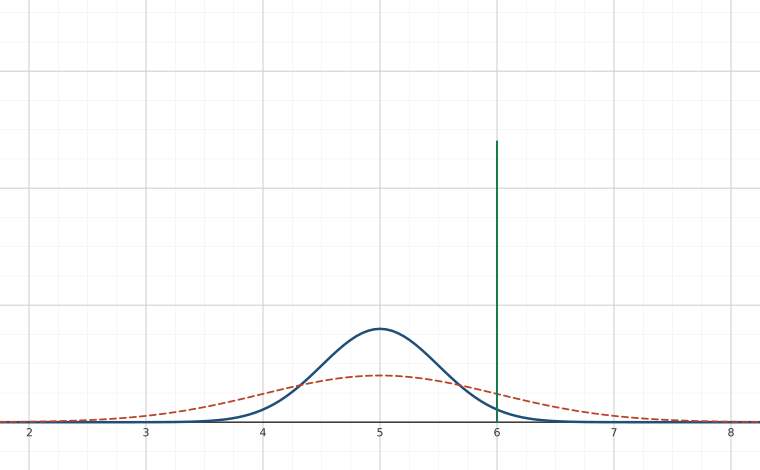
The lab's population - screw lengths, mean 5 inches, standard deviation 1 inch - is the dashed curve and never moves. The solid curve is the sampling distribution of the mean of n screws, with n on a slider, and the green line marks the 6 inches the lab asks about. The figure computes no probability: it shows why the two questions have such different answers. At n = 1 the curves coincide and 6 inches is only one standard deviation out. Drag n up and the solid curve pulls in around 5, because its standard deviation is 1/sqrt(n) - 0.5 at n = 4, 0.316 at the lab's n = 10 - until almost nothing is left beyond the green line. Read the picture first, then compute both probabilities and check that the numbers say what the shapes say.
The lengths of metal screws are normally distributed, with a mean of 5 inches, and standard deviation of 1 inch.
If 10 screws are chosen at random, what is the probability that their mean length is less than 6 inches?
If 10 screws are chosen at random, what is the probability that their mean length is between 5 and 6 inches?
Adapted from Python for Introductory Statistics: Student's Lab Workbook, by Simon Aman (Truman College, City Colleges of Chicago), licensed under CC BY 4.0. Changes were made: reformatted as an accessible XYZ web edition with live in-browser code cells. License: CC-BY-4.0.
These eBooks are a prerelease and are not yet certified conformant with WCAG 2.1 AA or ADA Title II. Every page is built against an automated accessibility gate, and the published editions will meet ADA Title II requirements when they release in late September 2026. If something is unusable, please tell us.