
Lab Answers
Lab 1.1.1
print("Hello, World")Show expected output
Hello, WorldLab 1.1.2
print('Welcome to Python Programming Language.')Show expected output
Welcome to Python Programming Language.Lab 1.2.1
10+10Show expected output
20Lab 1.2.2
100-88Show expected output
12Lab 1.2.3
1/2+7.1-10*3Show expected output
-22.4Lab 1.2.4
-5 + 7 - (100+.05)/10Show expected output
-8.004999999999999Lab 1.2.5
1/671000000Show expected output
1.4903129657228019e-09Lab 1.2.6
6.25*100*16000Show expected output
10000000.0Lab 1.2.7
28/4*2Show expected output
14.0Lab 1.2.8
7**2+1/2**(1/2)Show expected output
49.707106781186546Lab 1.2.9
7**2-8**(1/2)Show expected output
46.17157287525381Lab 1.2.10
(7**2-8**(1/2))/25Show expected output
1.8468629150101523Lab 1.3.1
x1 = 6
y1 = 9
x2 = 5
y2 = 1

m = (y2-y1)/(x2-x1)

x = (x1+x2)/2
y = (y1+y2)/2

print('slope is',m)
print('mid point is (',x,',',y,')')
Show expected output
slope is 8.0
mid point is ( 5.5 , 5.0 )
Lab 1.3.2
a = 2
b = -3
c = -4

x1 = -b-(b**2-4*a*c)**(1/2)
x1 = x1/(2*a)

x2 = -b+(b**2-4*a*c)**(1/2)
x2 = x2/(2*a)

print("one solution is ", x1)
print("another solution is ", x2)
Show expected output
one solution is  -0.8507810593582121
another solution is  2.350781059358212
Lab 1.3.3
round((1+2)/18,1)Show expected output
0.2OR
a = (1+2)/18
round(a,1)
Show expected output
0.2Lab 1.4.1
length = 5
width = 8
area = length*width  # the area of a rectangle is length times width
print(area)         # display the result
Show expected output
40Lab 1.5.1
abs(7*2-89**(1/2))Show expected output
4.566018867943397OR
a = 7*2-89**(1/2)
abs(a)
Show expected output
4.566018867943397Lab 1.5.2
(abs(7**2-8**(1/2)))/25Show expected output
1.8468629150101523OR
a = 7**2-8**(1/2)
b = abs(a)
b/25
Show expected output
1.8468629150101523Lab 1.5.3
import numpy as np

sin = np.sin(np.pi/3)

Area = 10*12*sin

print(Area)
Show expected output
103.92304845413263Lab 1.5.4
import numpy as np

np.sqrt(6**2-4*2*(-5))
Show expected output
8.717797887081348OR
import numpy as np

a = 6**2-4*2*(-5)
np.sqrt(a)
Show expected output
8.717797887081348Lab 1.6.1
# w=input("Enter weight in pounds:")  #ask the user for a number
w = "180"   # ← web edition: the value the book's own run typed in
# h1 = input("Enter height feet only:")
h1 = "5"   # ← web edition: the value the book's own run typed in
# h2 = input("Enter inches:")
h2 = "9"   # ← web edition: the value the book's own run typed in
w,h1,h2 = float(w),float(h1),float(h2) # converst the number to float
bmi = 703*(w/(h1*12+h2)**2)
print("The BMI is", bmi)
Show expected output
Enter weight in pounds:180
Enter height feet only:5
Enter inches:9
The BMI is 26.578449905482042
Lab 2.1.1
x = [1,2,3,4,5,6,7,8,9]
x
Show expected output
[1, 2, 3, 4, 5, 6, 7, 8, 9]Lab 2.1.2
x = [1,2,3,4,5,6,7,8,9]
x[0]
Show expected output
1Lab 2.1.3
x = [1,2,3,4,5,6,7,8,9]
x[-1]
Show expected output
9Lab 2.1.4
x = [1,2,3,4,5,6,7,8,9]
x[1:4]
Show expected output
[2, 3, 4]Lab 2.2.1
x = [72,82,66,70,66,60,53,56,49]

x.sort()
print(x)
Show expected output
[49, 53, 56, 60, 66, 66, 70, 72, 82]Lab 2.2.2
x = [72,82,66,70,66,60,53,56,49]

max(x)
Show expected output
82Lab 2.2.3
x = [72,82,66,70,66,60,53,56,49]

x.sort()
x.reverse()print(x)Show expected output
[82, 72, 70, 66, 66, 60, 56, 53, 49]Lab 3.1.1
a = 1   # coefficient of x^2
b = 3   # coefficient of x
c = 4  # constant term

d = b**2 - 4*a*c

if d < 0:
  print("No real solution")
elif d == 0:
  print("One real solution")
else:
  print("Two real solutions")
Show expected output
No real solutionLab 3.1.2
a = 5   # coefficient of x^2
b = 3   # coefficient of x
c = -16  # constant term

d = b**2 - 4*a*c

if d < 0:
  print("No real solution")
elif d == 0:
  print("One real solution")
else:
  print("Two real solutions")
Show expected output
Two real solutionsLab 3.2.1
def quadra(a,b,c):
  a,b,c = float(a),float(b),float(c)
  if b**2-4*a*c < 0:
    return print("No real solutions")
  elif b**2-4*a*c == 0:
    x1 = -b/(2*a)
    return print("the solution is", x1)
  else:
    x1 = (-b-(b**2-4*a*c)**.5)/(2*a)
    x2 = (-b+(b**2-4*a*c)**.5)/(2*a)
    return print("the solutions are: ",x1," and ",x2)
quadra(-1,-1,10) # in this case a=-1 b=-1 c=10Show expected output
the solutions are: 2.7015621187164243 and -3.7015621187164243Lab 3.2.2
def quadra(a,b,c):
  a,b,c = float(a),float(b),float(c)
  if b**2-4*a*c < 0:
    return print("No real solutions")
  elif b**2-4*a*c == 0:
    x1 = -b/(2*a)
    return print("the solution is", x1)
  else:
    x1 = (-b-(b**2-4*a*c)**.5)/(2*a)
    x2 = (-b+(b**2-4*a*c)**.5)/(2*a)
    return print("the solutions are: ",x1," and ",x2)
quadra(1,1,1) # heare a=1 b=1 c=1Show expected output
No real solutionsLab 3.3.1
b=2
 c=4
b/c
Show error output
  File "<ipython-input-86-158994d5983a>", line 2
    c=4
    ^
IndentationError: unexpected indent
Lab 3.3.2 if a > b:
a = 1
b = 2
if a > b
 print("a is bigger than b")
elif a = b:
 print("equal)
else:
 print("a is smaller than b")
Show error output
  File "<ipython-input-87-871e93d2a39b>", line 3
    if a > b
            ^
SyntaxError: invalid syntax
Lab 3.3.3
a = 1
b = 2
if a > b:
 print("a is bigger than b")
elif a = b:
 print("equal)
else:
 print("a is smaller than b"):
Show error output
  File "<ipython-input-88-128f45613308>", line 5
    elif a = b:
           ^
SyntaxError: invalid syntax
Lab 3.3.4
a = 1
b = 2
if a > b:
 print("a is bigger than b")
elif a == b:
 print("equal)
else:
 print("a is smaller than b")
Show error output
  File "<ipython-input-90-9aa3a9224cf2>", line 6
    print("equal)
                 ^
SyntaxError: EOL while scanning string literal
Lab 4.1.1
age = [77, 72,73,62,77,55]

sum = 0

for i in age:
  sum = sum + i

aver = sum/len(age)

print("The average age of IL Supreme Court Justices is ", aver)
Show expected output
The average age of IL Supreme Court Justices is 69.33333333333333Lab 4.2.1
n = 20

i = 0
a = 1
b = 1

while i < n:
    print (a)
    i = i + 1
    c = a + b
    a = b
    b = c
Show expected output
1
1
2
3
5
8
13
21
34
55
89
144
233
377
610
987
1597
2584
4181
6765
Lab 4.2.2
# n = input("Type in a maximum positive integer and press enter" )
n = "5"   # ← web edition: the value the book's own run typed in
n = int(n)

i = 1

while i < n+1:
  print(i)
  i = i+1
Show expected output
Type in a maximum positive integer and press enter5
1
2
3
4
5
Lab 4.2.3
# n = input("Tpye in a positive integer and press enter ")
n = "10"   # ← web edition: the value the book's own run typed in
n = int(n)

if n == 0 or n == 1:
 f = 1
elif n < 0:
 print("Error: non-negative integers only")
else:
  i = 1
  f = 1
  while i < n+1:
    f = f*i
    i = i + 1
  print("n factorial is",f)
Show expected output
Tpye in a positive integer and press enter 10
n factorial is 3628800
Lab 5.1.1
import numpy as np

x = [20, 21, 25, 20, 29, 25, 22, 25, 21, 25]

np.unique(x,return_counts=True)
Show expected output
(array([20, 21, 22, 25, 29]), array([2, 2, 1, 4, 1]))Lab 5.1.2
import numpy as np

x = ['NO', 'NO', 'YES', 'YES', 'NO', 'YES', 'NO', 'NO', 'YES', 'NO', 'YES',
     'NO', 'NO', 'YES', 'YES', 'YES', 'YES', 'NO', 'YES', 'YES']
np.unique(x,return_counts=True)
Show expected output
(array(['NO', 'YES'], dtype='<U3'), array([ 9, 11]))Lab 5.1.3
import numpy as np

x = [40,40,40,40,40,41,41,41,41,41,41,42,42,42,42,43,43,43,43,43,43,44,44,44,
     44,45]

freq,bin_edges = np.histogram(x,5,density=False)

print(bin_edges)
print(freq)
Show expected output
[40. 41. 42. 43. 44. 45.]
[5 6 4 6 5]
40 to 41 has 5 scores 41 to 42 has 6 scores 42 to 43 has 4 scores 43 to 44 has 6 scores 44 to 45 has 5 scores
| scores | freq |
|---|---|
| 40-41 | 5 |
| 41-42 | 6 |
| 42-43 | 4 |
| 43-44 | 6 |
| 44-45 | 5 |
Lab 5.3.1
import matplotlib.pyplot as plt


race = ['Latinx','Black','White','other']
death = [1859,2224,1233,309]

plt.bar(race,death)
Show expected output
<BarContainer object of 4 artists>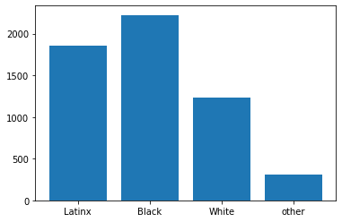
5.3.2
import matplotlib.pyplot as plt

race = ['Latinx','Black','White','other']
death = [1859,2224,1233,309]

plt.pie(death,labels=race,autopct='%1.1f%%')
Show expected output
([<matplotlib.patches.Wedge at 0x7fdd012ef410>,
  <matplotlib.patches.Wedge at 0x7fdd012efb50>,
  <matplotlib.patches.Wedge at 0x7fdd012f9410>,
  <matplotlib.patches.Wedge at 0x7fdd012f9d10>],
 [Text(0.5584906875918265, 0.9476751299222794, 'Latinx'),
  Text(-1.0828050332538752, -0.19373502512471624, 'Black'),
  Text(0.5627194086838145, -0.9451702847056388, 'White'),
  Text(1.0836598543140907, -0.18889499767850831, 'other')],
 [Text(0.3046312841409962, 0.5169137072303341, '33.0%'),
  Text(-0.5906209272293864, -0.10567365006802702, '39.5%'),
  Text(0.3069378592820806, -0.5155474280212574, '21.9%'),
  Text(0.5910871932622312, -0.10303363509736815, '5.5%')])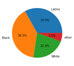
Lab 5.4.1
import matplotlib.pyplot as plt


x = [46776, 53736, 53736, 54840, 57408, 57408, 57408, 57408, 57408, 57408,
     60108, 60108, 62712, 63552, 66852, 66852, 69732, 70032, 70044, 70272,
     72024, 73380, 73380, 73380, 75408, 75468, 76248, 80484, 80484, 80484,
     82476, 82788, 82836, 83676, 84324, 84324, 84324, 85848, 87564, 88272,
     88272, 90828, 92004, 92304, 92520, 96060, 96096, 100680, 100716, 100716,
     103764, 105420, 109620, 146868]

plt.hist(x,bins=6,ec='k')
Show expected output
(array([13., 14., 20.,  6.,  0.,  1.]),
 array([ 46776.,  63458.,  80140.,  96822., 113504., 130186., 146868.]),
 <a list of 6 Patch objects>)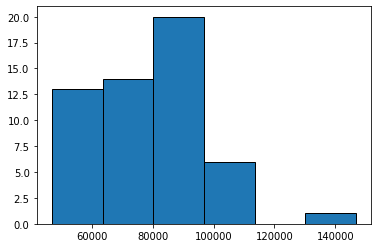
Lab 5.4.2
import matplotlib.pyplot as plt

x = [46776, 53736, 53736, 54840, 57408, 57408, 57408, 57408, 57408, 57408,
     60108, 60108, 62712, 63552, 66852, 66852, 69732, 70032, 70044, 70272,
     72024, 73380, 73380, 73380, 75408, 75468, 76248, 80484, 80484, 80484,
     82476, 82788, 82836, 83676, 84324, 84324, 84324, 85848, 87564, 88272,
     88272, 90828, 92004, 92304, 92520, 96060, 96096, 100680, 100716, 100716,
     103764, 105420, 109620, 146868]

freq,bins,_ = plt.hist(x,bins=6,ec='k')
plt.xticks(bins)
plt.title("Aviation Employee Salaries")
plt.xlabel("Salary")
plt.ylabel("Frequency")
Show expected output
Text(0, 0.5, 'Frequency')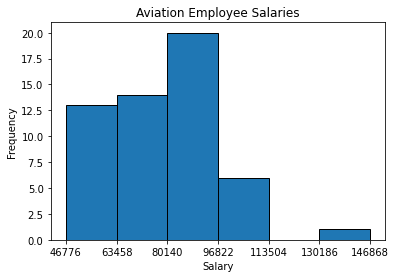
Lab 5.4.3
Copy, paste and run the polygon function below. Then write a Python code to call the function with the given data.
def polygon(x,n):
  import matplotlib.pyplot as plt
  import numpy as np

  freq, bins, edges = plt.hist(x,bins=n,ec="k",range=[min(x),max(x)+1])
  plt.title("Polygon")
  plt.xlabel('data values')
  plt.ylabel('frequency')

  a1=bins[0]-(bins[1]-bins[0])
  a2=bins[-1]+(bins[1]-bins[0])
  bin1=np.insert(bins,[0],a1)
  bin1=np.append(bin1,a2)

  freq,edges,_=plt.hist(x,bins=bin1,ec='k', range=[min(x),max(x)+1])
  midpoints=0.5*(edges[1:]+edges[:-1])
  plt.plot(midpoints,freq)
  plt.xticks(bin1)
  plt.show()
x = [46776, 53736, 53736, 54840, 57408, 57408, 57408, 57408, 57408, 57408,
60108, 60108, 62712, 63552, 66852, 66852, 69732, 70032, 70044, 70272,
72024, 73380, 73380, 73380, 75408, 75468, 76248, 80484, 80484, 80484,
82476, 82788, 82836, 83676, 84324, 84324, 84324, 85848, 87564, 88272,
88272, 90828, 92004, 92304, 92520, 96060, 96096, 100680, 100716, 100716,
103764, 105420, 109620, 146868]
polygon(x,6)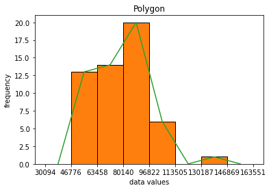
Lab 5.4.4
Copy the 'ogive' function, paste and run it below. Then use it to make an ogive.
def ogive(x,n):
  import matplotlib.pyplot as plt
  import numpy as np

  freq, bins, edges = plt.hist(x,bins=n,ec="k",range=[min(x),max(x)+1])
  plt.title("Ogive")
  plt.xlabel('data values')
  plt.ylabel('Cumulative frequency')

  a1=bins[0]-(bins[1]-bins[0])
  a2=bins[-1]+(bins[1]-bins[0])
  bin1=np.insert(bins,[0],a1)
  bin1=np.append(bin1,a2)

  freq,edges,_=plt.hist(x,bins=bin1,ec='k', range=[min(x),max(x)+1])

  ogive1 = edges[:-1]
  cumfreq = np.cumsum(freq)
  plt.plot(ogive1,cumfreq)
  plt.xticks(bin1)
  plt.show()
x = [46776, 53736, 53736, 54840, 57408, 57408, 57408, 57408, 57408, 57408,
60108, 60108, 62712, 63552, 66852, 66852, 69732, 70032, 70044, 70272,
72024, 73380, 73380, 73380, 75408, 75468, 76248, 80484, 80484, 80484,
82476, 82788, 82836, 83676, 84324, 84324, 84324, 85848, 87564, 88272,
88272, 90828, 92004, 92304, 92520, 96060, 96096, 100680, 100716, 100716,
103764, 105420, 109620, 146868]
ogive(x,6)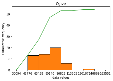
Lab 5.5.1
Copy the dotplots function and paste it below. Then use it to draw a dot plot.
# dotplot by Patrick FitzGerald
def dotplots(x,x_label="Data Values"):   # function name is dotplots takes a x

 import numpy as np
 import matplotlib.pyplot as plt

 data = np.array(x)   # convert to array
 values, counts = np.unique(data, return_counts=True)

# dot plot with appropriate figure size and y-axis limits
 fig, ax = plt.subplots(figsize=(6, 2.25))
 for value, count in zip(values, counts):
    ax.plot([value]*count, list(range(count)), 'co', ms=10, linestyle='')
 for spine in ['top', 'right', 'left']:
    ax.spines[spine].set_visible(False)
 ax.yaxis.set_visible(False)
 ax.set_ylim(-1, max(counts))
 ax.set_xticks(range(min(values), max(values)+1))
 ax.tick_params(axis='x', length=0, pad=8, labelsize=12)

 plt.suptitle("Dot Plot")
 plt.ylabel("frequency")
 plt.xlabel(x_label)

 return plt.show()
x = [6, 4, 4, 2, 1, 3, 5, 2, 4, 2, 5, 4, 4, 7, 4, 3, 4, 1, 2, 5]
dotplots(x, "Waiting Time")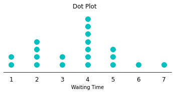
Lab 5.6.1
First install stemgraphic
pip install stemgraphicimport stemgraphic
x = [54, 22, 77, 92, 51, 68, 37, 27, 68, 47, 42, 38, 18, 46, 74, 77, 81, 78, 16,
35, 77, 90, 82, 36, 50, 39, 19, 62, 70, 88, 36, 37, 53, 72, 77]
stemgraphic.stem_graphic(x,scale=10,aggregation=False)Show expected output
(<Figure size 540x216 with 1 Axes>,
 <matplotlib.axes._axes.Axes at 0x7fefe45b7410>)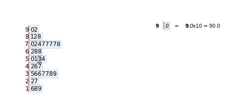
Lab 6.1.1
import numpy as np

x = [46776, 53736, 53736, 54840, 57408, 57408, 57408, 57408, 57408, 57408,
     60108, 60108, 62712, 63552, 66852, 66852, 69732, 70032, 70044, 70272,
     72024, 73380, 73380, 73380, 75408, 75468, 76248, 80484, 80484, 80484,
     82476, 82788, 82836, 83676, 84324, 84324, 84324, 85848, 87564, 88272,
     88272, 90828, 92004, 92304, 92520, 96060, 96096, 100680, 100716, 100716,
     103764, 105420, 109620, 146868]


print("mean and median")
print(np.mean(x))
print(np.median(x))
Show expected output
mean and median
78460.0
78366.0
Interpretation: The mean and median are 78460.0 and 78366.0 respectively.
Lab 6.2.1
import numpy as np

x=[75408, 82368, 103968, 82368, 42996, 85992, 67464, 103716, 134292, 113484,
   94848, 101628, 119712, 61776, 122496, 57720, 119712, 119712, 61140, 103716,
   67464, 58680, 91020, 83268, 62712, 78828, 82788, 91020, 75408, 59820, 79812,
   63348, 122496, 72744, 98628, 103968, 103968, 131664, 115788, 76248, 119712,
   83268, 75408, 75408, 95172, 67824, 75408, 119712, 141696, 97392, 83268,
   59820, 97668, 82368, 53736, 65676, 103716, 94848, 79020, 67824, 86856,
   103716, 75408, 119712, 91944, 94848, 66336, 99480, 119712]

print('the population variance and standared devaition are')
print(np.var(x,ddof=0))
print(np.std(x,ddof=0))
Show expected output
the population variance and standared devaition are
490101843.4177693
22138.24390998006
Lab 6.2.2
import numpy as np

x = [46776, 53736, 53736, 54840, 57408, 57408, 57408, 57408, 57408, 57408,
     60108, 60108, 62712, 63552, 66852, 66852, 69732, 70032, 70044, 70272,
     72024, 73380, 73380, 73380, 75408, 75468, 76248, 80484, 80484, 80484,
     82476, 82788, 82836, 83676, 84324, 84324, 84324, 85848, 87564, 88272,
     88272, 90828, 92004, 92304, 92520, 96060, 96096, 100680, 100716, 100716,
     103764, 105420, 109620, 146868]

print('The sample variance and standard deviation')
print(np.var(x,ddof=1))
print(np.std(x,ddof=1))
Show expected output
The sample variance and standard deviation
333192547.0188679
18253.562584297564
Interpretation: The sample variance and standard devation are 333192547.0188679 and 18253.562584297564 respectively.
Lab 6.4.3
import numpy as np

x = [5200, 7200, 9200, 11200, 13500]
f = [9,21,18,16,5]

np.average(x,weights=f)
Show expected output
8844.927536231884Interpretaton: The sample mean is 8844.927536231884
import numpy as np

x = [5200, 7200, 9200, 11200, 13500]
f = [9,21,18,16,5]

np.sqrt(np.cov(x,fweights=f,ddof=1))
Show expected output
2350.6905263250064Interpretation: The sample standard devition 2350.6905263250064
Lab 7.1.1
import numpy as np

x = [75408, 82368, 103968, 82368, 42996, 85992, 67464, 103716, 134292, 113484,
     94848, 101628, 119712, 61776, 122496, 57720, 119712, 119712, 61140, 103716,
     67464, 58680, 91020, 83268, 62712, 78828, 82788, 91020, 75408, 59820,
     79812, 63348, 122496, 72744, 98628, 103968, 103968, 131664, 115788, 76248,
     119712, 83268, 75408, 75408, 95172, 67824, 75408, 119712, 141696, 97392,
     83268, 59820, 97668, 82368, 53736, 65676, 103716, 94848, 79020, 67824,
     86856, 103716, 75408, 119712, 91944, 94848, 66336, 99480, 119712]

np.quantile(x,[.10,.25,.50,.75,.90])
Show expected output
array([ 61648.8, 75408. , 85992. , 103716. , 119712. ])Interpretation: The 10th, 25th, 50th, 75th and 90th percentile are 61648.8, 75408.0, 85992.0, 103716.0, and 119712.0 respectively.
Lab 7.2.1
import numpy as np
from scipy import stats

x = [46776, 53736, 53736, 54840, 57408, 57408, 57408, 57408, 57408, 57408,
       60108, 60108, 62712, 63552, 66852, 66852, 69732, 70032, 70044, 70272,
       72024, 73380, 73380, 73380, 75408, 75468, 76248, 80484, 80484, 80484,
       82476, 82788, 82836, 83676, 84324, 84324, 84324, 85848, 87564, 88272,
       88272, 90828, 92004, 92304, 92520, 96060, 96096, 100680, 100716, 100716,
       103764, 105420, 109620, 146868]

x_array = np.array(x)   # convert the list to a numpy array

stats.percentileofscore(x_array,80000,kind='rank')
Show expected output
50.0Interpretation: The percentile salary rank of an emplyee with salary 80000 is 50.
Lab 7.3.1
import matplotlib.pyplot as plt
x = [27.3, 5.5, 14.3, 3.2, 16.8, 17.9, 14.2, 14.2, 9.6, 34.7, 8.9, 30.1,
        27.7, 17.7, 21.8, 47.7, 37, 24.9]
plt.boxplot(x,vert=False,showmeans=True)
Show expected output
{'boxes': [<matplotlib.lines.Line2D at 0x7fdd00f4be90>],
 'caps': [<matplotlib.lines.Line2D at 0x7fdd00ed1f10>,
  <matplotlib.lines.Line2D at 0x7fdd00ed7490>],
 'fliers': [<matplotlib.lines.Line2D at 0x7fdd00ede490>],
 'means': [<matplotlib.lines.Line2D at 0x7fdd00ed7f50>],
 'medians': [<matplotlib.lines.Line2D at 0x7fdd00ed7a10>],
 'whiskers': [<matplotlib.lines.Line2D at 0x7fdd00ed1490>,
  <matplotlib.lines.Line2D at 0x7fdd00ed19d0>]}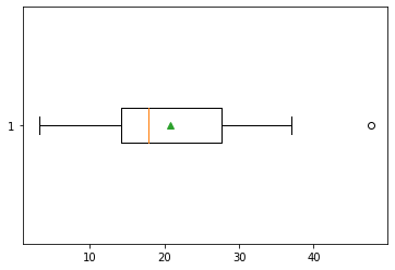
Lab 8.1.1
import numpy as np

x = [0, 1, 2, 3, 4, 5, 6, 7, 8]
p = [0.197, 0.212, 0.255,	0.182, 0.09, 0.04, 0.02, 0.003, 0.001]

average = np.average(x, weights=p)
std = np.sqrt(np.cov(x,aweights=p, ddof=0))

print('mean is',average)
print('standard deviation is',std)
Show expected output
mean is 1.977
standard deviation is 1.5272429407268509
Lab 8.2.1
from scipy import stats
stats.binom.pmf(1,30,.21)
Show expected output
0.006769026228180294from scipy import stats
stats.binom.cdf(4,30,.21)Show expected output
0.2145879371696642from scipy import stats
1-stats.binom.cdf(3,30,.21)Show expected output
0.9015599620024068Interpretation:
= 0.006769026228180294
= 0.2145879371696642
= 0.9015599620024068
Mean = 6.3 and std = 2.2309190931093847
Lab 8.2.2
# binomial graph with n and p
def binomplot(n,p):
  from scipy import stats
  import numpy as np
  import matplotlib.pyplot as plt

  x = np.arange(0,n+1)
  y = stats.binom.pmf(x,n,p)
  plt.bar(x,y,width=0.2)

  plt.suptitle("Binomial Plot")
  plt.xlabel("x values")
  plt.ylabel("probability")

  return plt.show()
binomplot(10,0.6)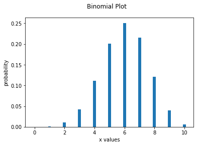
Lab 9.1.1
from scipy import stats
stats.uniform.cdf(15,5,15-5)
Show expected output
1.0Lab 9.2.1
from scipy import stats
stats.norm.cdf(1.5,0,1)
Show expected output
0.9331927987311419Lab 9.2.2
from scipy import stats
stats.norm.cdf(27726,27191,7126)
Show expected output
0.5299233487082249Interpretation: Probability that the average cost is less than $27726 is 0.5299233487082249
Lab 9.2.3
from scipy import stats
stats.norm.ppf(.75,27191,7126)
Show expected output
31997.413959897276Interpretation: 75 percent of the average college costs are less than or equal to 31997.413959897276
Lab 9.3.1
from scipy import stats
stats.norm.cdf(6,5,1/(10**.5))
Show expected output
0.9992172988709987Interpretation: The probabilty that the mean length is less than 6 is 0.9992172988709987. That is
from scipy import stats
stats.norm.cdf(6,5,1/(10**.5)) - stats.norm.cdf(5,5,1/(10**.5))
Show expected output
0.49921729887099875Interpretation: The probability that the average length is between 5 and 6 is 0.49921729887099875. That is,
Lab 10.1.1
# Confidence interval, given confidence level C, std, n
def conf_z_mean(C,mean,std,n):
     from scipy import stats
     ebm = (std/n**.5)*stats.norm.ppf(C+(1-C)/2,0,1)
return print("(", mean-ebm, ",", mean+ebm, ')')conf_z_mean(.90,80,15,50)Show expected output
( 76.51073853896997 , 83.48926146103003 )conf_z_mean(.90,80,15,50) Interpretation: The 90% confidence interval is.
Lab 10.2.1
# marigin of error given the level of confidence C, mean, std and n
def error_t_mean(C,std,n):
    from scipy import stats
    ebm = (std/n**.5)*stats.t.ppf(C+(1-C)/2,n-1,0,1)
return print("Margin of Error is",ebm)error_t_mean(.9,7,25)Show expected output
Margin of Error is 2.3952349118731986# confidence interval given level of confidence C and x
def conf_t_mean(C,mean,std,n):
from scipy import stats
ebm = (std/n**.5)*stats.t.ppf(C+(1-C)/2,n-1,0,1)
print ('mean is',mean,'and std is',std)
return print("(", mean-ebm, ",", mean+ebm, ')' )conf_t_mean(.9,85,7,25)Show expected output
mean is 85 and std is 7
( 82.6047650881268 , 87.3952349118732 )
Lab 10.3.1
# confidence interval and margin of error given p and n

def conf_prop_stats(C,p,n):
  from scipy import stats
  eb1 = ((p*(1-p)/n)**.5)*stats.norm.ppf(C+(1-C)/2,0,1)
  return print(" Sample Proportion =",p,"\n Margine of Error = ", eb1,
"\n Confidence Interval","(",p - eb1,",",p + eb1,")")p=51/120conf_prop_stats(.9,p,120)Show expected output
 Sample Proportion = 0.425
 Margine of Error =  0.07422753204362957
 Confidence Interval ( 0.3507724679563704 , 0.4992275320436296 )
Lab 10.3.2
# confidence interval and margin of error given p and n

def conf_prop(C,p,n):
  from scipy import stats
  eb1 = ((p*(1-p)/n)**.5)*stats.norm.ppf(C+(1-C)/2,0,1)
  return print(" Sample Proportion =",p,"\n Margine of Error = ", eb1,
"\n Confidence Interval","(",p - eb1,",",p + eb1,")")conf_prop(.95,.5,120)Show expected output
 Sample Proportion = 0.5
 Margine of Error =  0.08945970718585784
 Confidence Interval ( 0.41054029281414217 , 0.5894597071858578 )
Lab 10.3.3
def samp_pro(C,p,E):
  from scipy import stats
  sam = p*(1-p)*stats.norm.ppf(C+(1-C)/2,0,1)**2/E**2
return print("sample size = ", sam)samp_pro(.9,.55,.03)Show expected output
sample size = 744.0244498762386Interpretation: A sample of size 745 is needed.
Lab 11.1.1
# z test with alternative 'smaller' or 'greater' or 'two-sided'
def z_test_mean(null_mean,sigma,sample_mean,n,alternative='two-sided'):
    from scipy import stats
    z = (sample_mean-null_mean)/(sigma/n**.5)
    if alternative == 'smaller':
        pv = stats.norm.cdf(z,0,1)
    elif alternative == 'greater':
        pv = 1-stats.norm.cdf(z,0,1)
    elif alternative == 'two-sided':
        if z< 0:
            pv = 2*stats.norm.cdf(z,0,1)
        else: pv = 2*(1-stats.norm.cdf(z,0,1))
    else:
        print("alternative option error")
return print("z test statistic = ", z, "and p-value = ",pv)z_test_mean(2,.5,2.0,25,'smaller')Show expected output
z test statistic = 0.0 and p-value = 0.5Interpretation: Since the p-value 0.5 is not less than alpha, fail to reject the null hypothesis. There is not enough evidence to support the offcial's claim.
lab 11.2.1
import numpy as np

x=[2.5, 3.0, 1.5, 2.4, 2.6, 2.1, 1.8, 1.5, 1.7, 1.9, 3.2, 2.3, 2.0, 1.8, 1.2,
   1.5, 2.3, 2.5, 1.8, 2.2, 3.3, 2.3, 1.6, 2.5, 2.2]

mean = np.mean(x)
std = np.std(x,ddof=1)
# t test with alternative being 'smaller' or 'greater' or 'two-sided'
# (this helper is defined in the textbook's 11.2; the workbook calls it
# without defining it, so the web edition brings it along)
def t_test_mean(null_mean,sample_mean,sample_std,n,alternative='two-sided'):
from scipy import stats
t = (sample_mean-null_mean)/(sample_std/n**.5)
if alternative == 'smaller':
pv = stats.t.cdf(t,n-1,0,1)
elif alternative == 'greater':
pv = 1-stats.t.cdf(t,n-1,0,1)
elif alternative == 'two-sided':
if t< 0:
pv = 2*stats.t.cdf(t,n-1,0,1)
else: pv = 2*(1-stats.t.cdf(t,n-1,0,1))
else:
print("alternative option syntax error")
return print("t test statistic = ", t, " p-value = ",pv)
t_test_mean(1.5, mean, std, 25, 'two-sided')Show expected output
t test statistic = 6.006870493491006 p-value = 3.3502350138547854e-06Interpretation: Since the p-value is 3.3502350138547854e-06 less than alpha, reject the null hypothesis. There is enough evidence to not support the official's claim.
Lab 12.3.1
def z_test_prop(null_prop,x,n,alternative):  #altenative can only be "smaller"
                                               # or "greater" or "two-sided"
    from scipy import stats
    p = x/n
    z = (p-null_prop)/(null_prop*(1-null_prop)/n)**.5
    if alternative == 'smaller':
        pv = stats.norm.cdf(z,0,1)
    elif alternative == 'greater':
        pv = 1-stats.norm.cdf(z,0,1)
    elif alternative == 'two-sided':
        if z< 0:
            pv = 2*stats.norm.cdf(z,0,1)
        else: pv = 2*(1-stats.norm.cdf(z,0,1))
    else:
        print("altrnative option syntax error")
return print("z test statistic = ", z, " p-value = ",pv)z_test_prop(.5,510,1000,'greater')Show expected output
z test statistic = 0.6324555320336764 p-value = 0.2635446284327688Interpretation: The p-value 0.2635446284327688 is NOT less than 5%. Do not reject the null hypothesis. There is no enough evidence to support the president's claim.
Lab 12.1.1
import numpy as np

x=[1,0,3,5,14,7,4,16,9,10]
y=[17000,20000,15000,10000,5000,9000,10000,2000,8000,9000]

np.corrcoef(x,y)
Show expected output
array([[ 1.        , -0.93825489],
       [-0.93825489,  1.        ]])
Interpretation: The correlation coefficient is -0.93825489
import matplotlib.pyplot as plt

x=[1,0,3,5,14,7,4,16,9,10]
y=[17000,20000,15000,10000,5000,9000,10000,2000,8000,9000]

plt.scatter(x,y)
Show expected output
<matplotlib.collections.PathCollection at 0x7fa3d949c190>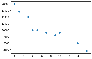
Lab 12.3.1
from scipy import stats

x=[1,0,3,5,14,7,4,16,9,10]
y=[17000,20000,15000,10000,5000,9000,10000,2000,8000,9000]

stats.linregress(x,y)
Show expected output
LinregressResult(slope=-955.6247567146751, intercept=17093.81082133126, rvalue=-0.9382548923679298, pvalue=5.899842619735838e-05, stderr=124.57425008729852)Interpretation: slope=-955.6247567146751, intercept=17093.81082133126, rvalue=-0.9382548923679298, pvalue=5.899842619735838e-05
Lab 12.3.1 (Alternative Solution Using Array)
from scipy import stats

x=[1,0,3,5,14,7,4,16,9,10]
y=[17000,20000,15000,10000,5000,9000,10000,2000,8000,9000]

results = stats.linregress(x,y) # save results as an arry named results

print('slope =', results[0]) # results[0] is the slope
print('intercept =', results[1]) # results[1] is the intercept
print('r =', results[2]) # results[2] is the r correlation-coefficient
print('p-value =', results[3]) # results[3] is p-value for testing pop. cor. co
Show expected output
slope = -955.6247567146751
intercept = 17093.81082133126
r = -0.9382548923679298
p-value = 5.899842619735838e-05
Interpretation: slope=-955.6247567146751, intercept=17093.81082133126, rvalue=-0.9382548923679298, pvalue=5.899842619735838e-05
import matplotlib.pyplot as plt
import numpy as np


x=[1,0,3,5,14,7,4,16,9,10]
y=[17000,20000,15000,10000,5000,9000,10000,2000,8000,9000]

x = np.array(x)
y = np.array(y)

y_hat = -955.6247567146751*x+17093.81082133126

plt.scatter(x,y)
plt.plot(x,y_hat)
Show expected output
[<matplotlib.lines.Line2D at 0x7fa3d9247f90>]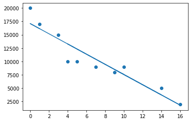
Lab 13.1.1
import numpy as np
from scipy import stats

obs = [306,232]
sum = np.sum(obs)
exp = [.513*sum,.469*sum]

stats.chisquare(obs,exp)
Show expected output
Power_divergenceResult(statistic=4.89897772395255, pvalue=0.026872598995409867)Interpretation: Since the p-value 0.026872598995409867 is less than , reject the null-hypothesis. There is enough evidence to reject the official's claim.
Lab 13.2.1
def chi2_test_of_indp(obs):
    from scipy import stats
    chi2, p, dof, ex = stats.chi2_contingency(obs)

    print("chi-square test statitic:",chi2)
    print("p-value:", p)
r1 = [1734,475,1281]
r2 = [2071,373,1938]
r3 = [678,103,935]
r4 = [534,92,560]
r5 = [5644,1661,2613]
r6 = [4094,927,1277]
obs = [r1,r2,r3,r4,r5,r6]
chi2_test_of_indp(obs)Show expected output
chi-square test statitic: 1509.7409528009978
p-value: 0.0
Interpretation: Since the p-value=0.0 is less than the level of significance, reject the null hypothesis. That is, there is enough evidence that race and crime-class are NOT independent.
Lab 14.1.1
import pandas as pd

x = ['male','female','female','male','male']
x_pd = pd.DataFrame({'gender':x})
print(x_pd)
Show expected output
   gender
0    male
1  female
2  female
3    male
4    male
Lab 14.1.2
import pandas as pd
x=[20, 21, 25, 20, 29, 25, 22, 25, 21, 25]
x_df=pd.DataFrame({'data':x})
x_df.value_counts(sort=False)
Show expected output
data
20      2
21      2
22      1
25      4
29      1
dtype: int64| data | freq |
|---|---|
| 20 | 2 |
| 21 | 2 |
| 22 | 1 |
| 25 | 4 |
| 29 | 1 |
Lab 14.1.3
import pandas as pd
x=[20, 21, 25, 20, 29, 25, 22, 25, 21, 25]
x_df=pd.DataFrame({'data':x})
x_df.value_counts(sort=False,normalize=True)
Show expected output
data
20      0.2
21      0.2
22      0.1
25      0.4
29      0.1
dtype: float64
Lab 14.1.4
import pandas as pd
x=['NO', 'NO', 'YES', 'YES', 'NO', 'YES', 'NO', 'NO', 'YES', 'NO', 'YES', 'NO',
   'NO', 'YES', 'YES', 'YES', 'YES', 'NO', 'YES', 'YES']

x_df = pd.DataFrame({'vote':x})
x_df.value_counts(normalize=True)
Show expected output
vote
YES     0.55
NO      0.45
dtype: float64
Lab 14.1.5
import pandas as pd
x = [46776, 53736, 53736, 54840, 57408, 57408, 57408, 57408, 57408, 57408,
     60108, 60108, 62712, 63552, 66852, 66852, 69732, 70032, 70044, 70272,
     72024, 73380, 73380, 73380, 75408, 75468, 76248, 80484, 80484, 80484,
     82476, 82788, 82836, 83676, 84324, 84324, 84324, 85848, 87564, 88272,
     88272, 90828, 92004, 92304, 92520, 96060, 96096, 100680, 100716, 100716,
     103764, 105420, 109620, 146868]

x_df = pd.DataFrame({'data':x})

x_df.describe()| data | |
|---|---|
| count | 54.000000 |
| mean | 78460.000000 |
| std | 18253.562584 |
| min | 46776.000000 |
| 25% | 64377.000000 |
| 50% | 78366.000000 |
| 75% | 88272.000000 |
| max | 146868.000000 |
Lab 14.1.6
import pandas as pd
x = [46776, 53736, 53736, 54840, 57408, 57408, 57408, 57408, 57408, 57408,
     60108, 60108, 62712, 63552, 66852, 66852, 69732, 70032, 70044, 70272,
     72024, 73380, 73380, 73380, 75408, 75468, 76248, 80484, 80484, 80484,
     82476, 82788, 82836, 83676, 84324, 84324, 84324, 85848, 87564, 88272,
     88272, 90828, 92004, 92304, 92520, 96060, 96096, 100680, 100716, 100716,
     103764, 105420, 109620, 146868]

x_df = pd.DataFrame({'salary':x})
print('skewness index is ',x_df.skew())
print('kurtosis index is',x_df.kurtosis())
Show expected output
skewness index is  salary    0.924462
dtype: float64
kurtosis index is salary    2.250167
dtype: float64
Lab 14.2.1
Data: Download data.csv (CSV, 16 KB)
import pandas as pd

url = 'data.csv'

x_df = pd.read_csv(url)

x_df.info()
Show expected output
<class 'pandas.core.frame.DataFrame'>
RangeIndex: 120 entries, 0 to 119
Data columns (total 14 columns):
 #   Column             Non-Null Count  Dtype
---  ------             --------------  -----
 0   valid_import       120 non-null    bool
 1   item               120 non-null    object
 2   importer_id        120 non-null    int64
 3   exporter_id        120 non-null    int64
 4   country_of_origin  120 non-null    object
 5   declared_quantity  120 non-null    int64
 6   declared_cost      120 non-null    float64
 7   mode_of_transport  120 non-null    object
 8   route              120 non-null    object
 9   date_of_departure  120 non-null    object
 10  date_of_arrival    120 non-null    object
 11  declared_weight    120 non-null    float64
 12  actual_weight      120 non-null    float64
 13  days_in_transit    120 non-null    float64
dtypes: bool(1), float64(4), int64(3), object(6)
memory usage: 12.4+ KB
Interpretation: for x_df
- class type is Pandas Dataframe
- 120 entries from 0 to 119
- 14 Columns
- Info for each Column listed
Lab 14.3.1
import pandas as pd

url = 'data.csv'

x_df = pd.read_csv(url)

x_df.describe()| importer_id | exporter_id | declared_quantity | declared_cost | declared_weight | actual_weight | days_in_transit | |
|---|---|---|---|---|---|---|---|
| count | 120.0 | 120.0 | 120.000000 | 120.000000 | 120.000000 | 120.000000 | 120.000000 |
| mean | 111.0 | 222.0 | 127.458333 | 6743.649881 | 1264.702934 | 1306.429806 | 35.424705 |
| std | 0.0 | 0.0 | 14.641311 | 2991.797050 | 633.149971 | 656.911704 | 26.571591 |
| min | 111.0 | 222.0 | 100.000000 | 1441.012419 | 18.459509 | 19.275241 | 12.410325 |
| 25% | 111.0 | 222.0 | 115.750000 | 4442.903914 | 820.314400 | 841.763738 | 18.225625 |
| 50% | 111.0 | 222.0 | 131.500000 | 6010.218745 | 1255.597743 | 1305.716419 | 27.044293 |
| 75% | 111.0 | 222.0 | 139.000000 | 8887.095370 | 1711.314045 | 1763.681083 | 44.356374 |
| max | 111.0 | 222.0 | 149.000000 | 14281.325362 | 2806.338955 | 2918.681683 | 147.787560 |
Interpretatoin: The descriptive statistics for importer_id and exporter_id are meaningless and should be ignored.
Lab 14.3.2
import pandas as pd

url = 'data.csv'

x_df = pd.read_csv(url)

x_df.groupby(['country_of_origin']).agg({'actual_weight':['mean','std','size']})| actual_weight | |||
|---|---|---|---|
| mean | std | size | |
| country_of_origin | |||
| China | 1307.147246 | 627.380399 | 24 |
| France | 1218.459074 | 728.100019 | 24 |
| India | 1304.722531 | 493.478451 | 24 |
| Italy | 1190.657039 | 711.818853 | 24 |
| USA | 1511.163138 | 702.116897 | 24 |
Lab 14.3.3
import pandas as pd

url = 'data.csv'

x_df = pd.read_csv(url)

x_df.groupby(['country_of_origin','route']).agg({'actual_weight':['mean','std','size']})| actual_weight | ||||
|---|---|---|---|---|
| mean | std | size | ||
| country_of_origin | route | |||
| China | america | 1281.081635 | 873.244407 | 6 |
| asia | 1492.969412 | 577.826149 | 6 | |
| europe | 1155.582715 | 465.171493 | 6 | |
| panama | 1298.955222 | 654.115536 | 6 | |
| France | america | 1142.095755 | 686.692379 | 6 |
| asia | 1218.311778 | 936.931509 | 6 | |
| europe | 1062.014711 | 756.490150 | 6 | |
| panama | 1451.414052 | 644.548543 | 6 | |
| India | america | 1007.777832 | 495.847993 | 6 |
| asia | 1697.493097 | 254.063822 | 6 | |
| europe | 1379.484100 | 516.208468 | 6 | |
| panama | 1134.135095 | 459.075799 | 6 | |
| Italy | america | 1035.376749 | 923.534914 | 6 |
| asia | 1512.269050 | 974.452899 | 6 | |
| europe | 1002.642317 | 461.640254 | 6 | |
| panama | 1212.340040 | 345.152024 | 6 | |
| USA | america | 1352.550563 | 895.589850 | 6 |
| asia | 1730.803390 | 725.189852 | 6 | |
| europe | 1445.528489 | 666.483253 | 6 | |
| panama | 1515.770109 | 634.190270 | 6 |
Lab 14.3.4
import pandas as pd

url = 'data.csv'

x_df = pd.read_csv(url)

x_df.boxplot(column=['actual_weight'],by=['country_of_origin'],showmeans=True,vert=False,rot=45)
Show expected output
<matplotlib.axes._subplots.AxesSubplot at 0x7f98bff49a90>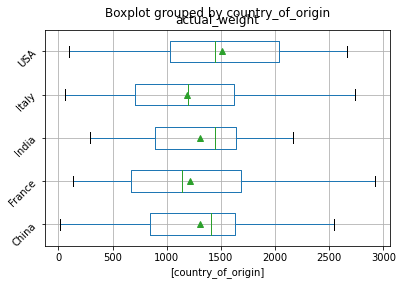
Lab 14.3.4 Alternative Solution
import pandas as pd
import seaborn as sns
sns.set_theme(style="ticks", palette="pastel")

# Load the example tips dataset
url = 'data.csv'

x_df = pd.read_csv(url)

sns.boxplot(x="actual_weight", y="country_of_origin", hue_order="smoker", palette=["m", "g"], data=x_df)
sns.despine(offset=10, trim=True)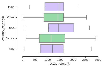
Lab 14.4.1
Data: Download my_csv_file.csv (CSV, 7 KB)
import pandas as pd

url='my_csv_file.csv'

x_df = pd.read_csv(url)
x_df.groupby(['section']).size().plot(kind='bar')

import matplotlib.pyplot as plt

plt.suptitle("Bar Graph")
plt.ylabel("Frequency")
Show source-edition output (different dataset)
Text(0, 0.5, 'Frequency')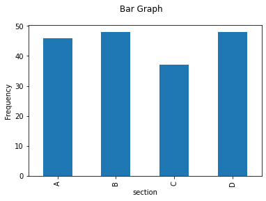
Lab 14.4.2
import pandas as pd

url='my_csv_file.csv'

x_df = pd.read_csv(url)
x_df.groupby(['section']).size().plot(kind='pie')

import matplotlib.pyplot as plt

plt.suptitle("Pie Chart")
plt.ylabel("sections")
Show source-edition output (different dataset)
Text(0, 0.5, 'sections')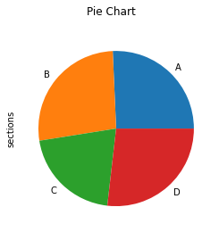
Lab 14.5.1
Data: Download kc_house_data.csv (CSV, 2.4 MB)
import pandas as pd

url = 'kc_house_data.csv'

x_df = pd.read_csv(url)
import statsmodels.formula.api as smf
model = smf.ols(formula='price ~ bedrooms + sqft_basement + sqft_living', data=x_df)
results = model.fit()
print(results.summary())Show expected output
                            OLS Regression Results
==============================================================================
Dep. Variable:                  price   R-squared:                       0.508
Model:                            OLS   Adj. R-squared:                  0.508
Method:                 Least Squares   F-statistic:                     7426.
Date:                Wed, 11 Aug 2021   Prob (F-statistic):               0.00
Time:                        13:38:08   Log-Likelihood:            -2.9995e+05
No. Observations:               21613   AIC:                         5.999e+05
Df Residuals:                   21609   BIC:                         5.999e+05
Df Model:                           3
Covariance Type:            nonrobust
=================================================================================
                    coef    std err          t      P>|t|      [0.025      0.975]
---------------------------------------------------------------------------------
Intercept      8.547e+04   6673.321     12.807      0.000    7.24e+04    9.85e+04
bedrooms      -5.806e+04   2312.155    -25.111      0.000   -6.26e+04   -5.35e+04
sqft_basement    26.6854      4.409      6.053      0.000      18.044      35.327
sqft_living     308.9346      2.478    124.668      0.000     304.077     313.792
==============================================================================
Omnibus:                    14369.246   Durbin-Watson:                   1.985
Prob(Omnibus):                  0.000   Jarque-Bera (JB):           489010.614
Skew:                           2.718   Prob(JB):                         0.00
Kurtosis:                      25.660   Cond. No.                     9.07e+03
==============================================================================

Warnings:
[1] Standard Errors assume that the covariance matrix of the errors is correctly specified.
[2] The condition number is large, 9.07e+03. This might indicate that there are
strong multicollinearity or other numerical problems.
Interpretation:
- See
x_df.headabove - where
- The F-statistic is 7426 with p-value of Prob (F-statistic) 0.00. Thus, the model has a significant contiribution to the prediction of price.
- The coefficient of determination (R-squared:) is 0.508.
- The p-value (P>|t|) for the
sqft_livingis 0.000 which is less than . It is significant.
Lab 14.5.2
Data: Download heart.csv (CSV, 25 KB)
import pandas as pd
df = pd.read_csv('heart.csv')
df.head()| row.names | sbp | tobacco | ldl | adiposity | famhist | typea | obesity | alcohol | age | chd | |
|---|---|---|---|---|---|---|---|---|---|---|---|
| 0 | 1 | 160 | 12.00 | 5.73 | 23.11 | Present | 49 | 25.30 | 97.20 | 52 | 1 |
| 1 | 2 | 144 | 0.01 | 4.41 | 28.61 | Absent | 55 | 28.87 | 2.06 | 63 | 1 |
| 2 | 3 | 118 | 0.08 | 3.48 | 32.28 | Present | 52 | 29.14 | 3.81 | 46 | 0 |
| 3 | 4 | 170 | 7.50 | 6.41 | 38.03 | Present | 51 | 31.99 | 24.26 | 58 | 1 |
| 4 | 5 | 134 | 13.60 | 3.50 | 27.78 | Present | 60 | 25.99 | 57.34 | 49 | 1 |
import statsmodels.formula.api as smf
model = smf.logit(formula='chd ~ ldl + age + sbp', data=df)
results = model.fit()

print(results.summary())
Show expected output
Optimization terminated successfully.
         Current function value: 0.553757
         Iterations 6
                           Logit Regression Results
==============================================================================
Dep. Variable:                    chd   No. Observations:                  462
Model:                          Logit   Df Residuals:                      458
Method:                           MLE   Df Model:                            3
Date:                Wed, 11 Aug 2021   Pseudo R-squ.:                  0.1416
Time:                        14:09:16   Log-Likelihood:                -255.84
converged:                       True   LL-Null:                       -298.05
Covariance Type:            nonrobust   LLR p-value:                 3.427e-18
==============================================================================
                 coef    std err          z      P>|z|      [0.025      0.975]
------------------------------------------------------------------------------
Intercept     -4.7372      0.768     -6.170      0.000      -6.242      -3.233
ldl            0.1863      0.053      3.487      0.000       0.082       0.291
age            0.0559      0.009      6.036      0.000       0.038       0.074
sbp            0.0048      0.005      0.898      0.369      -0.006       0.015
==============================================================================
Interpretation:
- Since LLR p-value 3.427e-18 is less than level of significance, the model contributes significantly to the prediction of
chd.
Lab 14.6.1
import pandas as pd

url='my_csv_file.csv'

x_df = pd.read_csv(url)
x_df.groupby(['level']).agg({'test3_score': ['mean', 'std','size']})| test3_score | |||
|---|---|---|---|
| mean | std | size | |
| level | |||
| high | 53.773333 | 3.184170 | 60 |
| low | 53.750000 | 2.329727 | 60 |
| medium | 53.831667 | 2.536546 | 60 |
import statsmodels.api as sm
from statsmodels.formula.api import ols
model = ols('test3_score ~ C(level)',data = x_df).fit()
table = sm.stats.anova_lm(model,type=1) # type 2 for equal or non-equal sample sizes
print(table)
Show source-edition output (different dataset)
             df       sum_sq   mean_sq         F    PR(>F)
C(level)    2.0     0.212333  0.106167  0.014477  0.985629
Residual  177.0  1298.037167  7.333543       NaN       NaN
Interpretation: Since the p-value 0.985629 is not less than = 0.10, we fail to reject the null hypothesis that the averages for all three levels are equal. That is, there is no significant difference between the averages of test3_score of the three levels.
Lab 14.6.2
import pandas as pd

url='my_csv_file.csv'

x_df = pd.read_csv(url)
x_df.groupby(['level','gender']).agg({'test3_score': ['mean', 'std','size']})| test3_score | ||||
|---|---|---|---|---|
| mean | std | size | ||
| level | gender | |||
| high | female | 54.036000 | 3.487463 | 25 |
| male | 53.585714 | 2.986946 | 35 | |
| low | female | 53.857576 | 2.521412 | 33 |
| male | 53.618519 | 2.111696 | 27 | |
| medium | female | 53.604167 | 2.688863 | 24 |
| male | 53.983333 | 2.456769 | 36 |
import statsmodels.api as sm
from statsmodels.formula.api import ols
model = ols('test3_score ~ C(level) + C(gender)',data = x_df).fit()
table = sm.stats.anova_lm(model,type=1) # type 2 for non-equal sample sizes
print(table)
Show source-edition output (different dataset)
              df       sum_sq   mean_sq         F    PR(>F)
C(level)     2.0     0.212333  0.106167  0.014401  0.985704
C(gender)    1.0     0.494704  0.494704  0.067102  0.795906
Residual   176.0  1297.542462  7.372400       NaN       NaN
Interpretation: There is no significant difference of the test3_score means between the three levles afte blocking by gender. No significant difference in the average test3_score between the two genders.
Lab 14.6.3
import pandas as pd

url='my_csv_file.csv'

x_df = pd.read_csv(url)
x_df.head()| id | gender | section | time | level | test1_score | test2_score | test3_score | |
|---|---|---|---|---|---|---|---|---|
| 0 | 1 | female | C | 17.3 | low | 65.4 | 84.3 | 51.9 |
| 1 | 2 | female | D | 5.1 | low | 72.4 | 86.1 | 52.0 |
| 2 | 3 | female | A | 2.4 | low | 73.8 | 84.2 | 53.1 |
| 3 | 4 | female | A | 8.8 | low | 70.2 | 87.9 | 52.0 |
| 4 | 5 | male | B | 15.0 | low | 60.3 | 81.4 | 55.5 |
x_df.groupby(['level','section']).agg({'test3_score': ['mean', 'std','size']})| test3_score | ||||
|---|---|---|---|---|
| mean | std | size | ||
| level | section | |||
| high | A | 54.207143 | 3.816657 | 14 |
| B | 52.538462 | 2.417484 | 13 | |
| C | 54.146667 | 3.044636 | 15 | |
| D | 54.105882 | 3.362192 | 17 | |
| low | A | 54.000000 | 1.942384 | 15 |
| B | 53.618750 | 1.880858 | 16 | |
| C | 53.750000 | 2.469548 | 16 | |
| D | 53.623077 | 3.181235 | 13 | |
| medium | A | 53.982353 | 2.444441 | 17 |
| B | 53.126316 | 1.659264 | 19 | |
| C | 53.250000 | 2.962938 | 6 | |
| D | 54.627778 | 3.136841 | 18 |
from statsmodels.formula.api import ols
model = ols('test3_score ~ C(level)*C(section)',data = x_df).fit()
table = sm.stats.anova_lm(model,type=2) # type 2 for non-equal sample sizes
print(table)
Show source-edition output (different dataset)
                        df       sum_sq    mean_sq         F    PR(>F)
C(level)               2.0     0.200742   0.100371  0.013460  0.986631
C(section)             3.0    31.217036  10.405679  1.395460  0.246013
C(level):C(section)    6.0    19.884361   3.314060  0.444434  0.848150
Residual             167.0  1245.286911   7.456808       NaN       NaN
Interpretation: There is no significant interaction effect between level and section of the average test3_score. 0.848150 > 0.10
Adapted from Python for Introductory Statistics: Student's Lab Workbook, by Simon Aman (Truman College, City Colleges of Chicago), licensed under CC BY 4.0. Changes were made: reformatted as an accessible XYZ web edition with live in-browser code cells. License: CC-BY-4.0.