9.2 Normal Probability Distribution

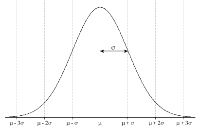
The normal probability distribution with mean $μ$ and standard deviation $σ$ is given by:

$f (x) = \frac{1}{σ \sqrt{2 π}} e^{- \frac{(x - μ)^{2}}{2 σ^{2}}}$ It is bell shaped and is symmetric about the mean $μ$ .

The normal curve: a bell-shaped density symmetric about the mean, with tick marks at μ − 3σ through μ + 3σ and a horizontal arrow marking one standard deviation σ from the mean to μ + σ.

The syntax for the normal cumulative probability $P (X < x)$ with $μ$ =mean and $σ$ =std is:

from scipy import stats
stats.norm.cdf(x,mean,std)

The syntax for inverse normal or p $^{t h}$ percentile (with area to the left of p) and $μ$ =mean and $σ$ =std is:

from scipy import stats
stats.norm.ppf(p,mean,std)

Note: The standard normal distribution has a mean $μ$ of zero and standard deviation $σ$ of one.

Example: In a standard normal distribution what is the probability that the z value is less than 2?

Watch demo video

from scipy import stats
stats.norm.cdf(2,0,1)    #for standard normal mean is zero and std is one

Show expected output

0.9772498680518208

Interpretation: $P open parenthesis z less than 2 close parenthesis equals 0.9772498680518208$

Example: In a standard normal distribution what is the probability that the z value is between -2 and 2.

$P (- 2 < z < 2) = P (z < 2) - P (z < - 2)$

=stats.norm.cdf(2,0,1)-stats.norm.cdf(-2,0,1)

from scipy import stats
stats.norm.cdf(2,0,1)-stats.norm.cdf(-2,0,1)

Show expected output

0.9544997361036416

Interpretation: $P (- 2 < z < 2) = 0.9544997361036416$

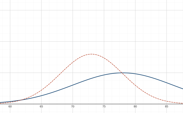
Example: The midterm exam scores in a math class is normally distributed with a mean of 73 and a standard deviation of 5.

Find the probability that a randomly selected student scored more than 65 on the exam.

$P (X > 65) = 1 - P (X < 65)$ =1-stats.norm.cdf(65,73,5)

Watch demo video

from scipy import stats
1-stats.norm.cdf(65,73,5)

Show expected output

0.945200708300442

Interpretation: $P open parenthesis X greater than 65 close parenthesis equals 0.945200708300442$

Example: The midterm exam scores in a math class is normally distributed with a mean of 73 and a standard deviation of 5.

Find the probability that a randomly selected student scored less than 85.

$P open parenthesis X less than 85 close parenthesis$ =stats.norm.cdf(85,73,5)

from scipy import stats
stats.norm.cdf(85,73,5)

Show expected output

0.9918024640754038

Interpretation: $P open parenthesis X less than 85 close parenthesis equals 0.9918024640754038$

Example: The midterm exam scores in a math class is normally distributed with a mean of 73 and a standard deviation of 5.

Find the 90th percentile (that is, find the score k that has 90% of the scores below k and 10% of the scores above k).

$90 to the power t h percentile$ = stats.norm.ppf(.9,73,5)

Watch demo video

from scipy import stats
stats.norm.ppf(.90,73,5)

Show expected output

79.407757827723

Interpretation: Ninety percent of scores are less than or equal to 79.407757827723

Example: The midterm exam scores in a math class is normally distributed with a mean of 73 and a standard deviation of 5.

Find the probability that a randomly selected student has a score between 70 and 90.

$P (70 < X < 90) = P (X < 90) - P (X < 70)$

stats.norm.cdf(90,73,5) - stats.norm.cdf(70,73,5)

Show expected output

0.7254099529842495

Interpretation: $P open parenthesis 70 less than X less than 90 close parenthesis equals 0.7254099529842495$

SciPy.Stats Summary of Probability Distributions

from scipy import stats

procedure	scipy.stats
Binomial pdf $P (X = x)$	`stats.binom.pmf(k,n,p)`
Binomial cdf $P (X \leq x)$	`stats.binom.cdf(k,n,p)`
Normal cdf $P (X \leq x)$	`stats.norm.cdf(x,mean,std)`
Inverse Normal or p-th Percentile	`stats.norm.ppf(p,mean,std)`
t distribution cdf $P (X \leq x)$	`stats.t.cdf(t,df,0,1)`
Inverse t or p-th Percentile	`stats.t.ppf(p,df,0,1)`
chi-square cdf $P open parenthesis χ squared less than or equal to c h 2 close parenthesis$	`stats.chi2.cdf(ch2,k-1)`
Inverse chi-square or p-th Percentile	`stats.chi2.ppf(p,k-1)`

Adapted from Python for Introductory Statistics, by Simon Aman (Truman College, City Colleges of Chicago), licensed under CC BY 4.0. Changes were made: reformatted as an accessible XYZ web edition with live in-browser code cells. License: CC-BY-4.0.