3.5 Discrete and Continuous Probability Distributions

Learning Outcomes

By the end of this section, you should be able to:

Describe fundamental aspects of probability distributions.
Apply discrete probability distributions including binomial and Poisson distributions.
Apply continuous probability distributions including exponential and normal distributions.
Use Python to apply various probability distributions for probability applications.

Probability distributions are used to model various scenarios to help with probability analysis and predictions, and they are used extensively to help formulate probability-based decisions. For example, if a doctor knows that the weights of newborn infants follow a normal (bell-shaped) distribution, the doctor can use this information to help identify potentially underweight newborn infants, which might indicate a medical condition warranting further investigation. Using a normal distribution, the doctor can calculate that only a small percentage of babies have weights below a certain threshold, which might prompt the doctor to further investigate the cause of the low weight. Or a medical researcher might be interested in the probability that a person will have high blood pressure or the probability that a person will have type O blood.

Overview of Probability Distributions

To begin our discussion of probability distributions, some terminology will be helpful:

Random variable—a variable where a single numerical value is assigned to a specific outcome from an experiment. Typically the letter $x$ is used to denote a random variable. For example, assign the numerical values 1, 2, 3, … 13 to the cards selected from a standard 52-card deck of Ace, 2, 3, … 10, Jack, Queen, King. Notice we cannot use “Jack” as the value of the random variable since by definition a random variable must be a numerical value.
Discrete random variable—a random variable is considered discrete if there is a finite or countable number of values that the random variable can take on. (If there are infinitely many values, the number of values is countable if it possible to count them individually.) Typically, a discrete random variable is the result of a count of some kind. For example, if the random variable $x$ represents the number of cars in a parking lot, then the values that x can take on can only be whole numbers since it would not make sense to have $x equals 15.37$ cars in the parking lot.
Continuous random variable—a random variable is considered continuous if the value of the random variable can take on any value within an interval. Typically, a continuous random variable is the result of a measurement of some kind. For example, if the random variable $x$ represents the weight of a bag of apples, then $x$ can take on any value such as $x equals 2.45734$ pounds of apples.

To summarize, the difference between discrete and continuous probability distributions has to do with the nature of the random variables they represent. Discrete probability distributions are associated with variables that take on a finite or countably infinite number of distinct values. Continuous probability distributions deal with random variables that can take on any value within a given range or interval. It is important to identify and distinguish between discrete and continuous random variables since different statistical methods are used to analyze each type.

Example 1

A coin is flipped three times. Determine a possible random variable that can be assigned to represent the number of heads observed in this experiment.

One possible random variable assignment could be to let $x$ count the number of heads observed in each possible outcome in the sample space. When flipping a coin three times, there are eight possible outcomes, and $x$ will be the numerical count corresponding to the number of heads observed for each outcome. Notice that the possible values for the random variable $x$ are 0, 1, 2 and 3, as shown in Table 3.3.

**Table 3.3**
Result for Flip #1	Result for Flip #2	Result for Flip #3	Value of Random Variable $x$
Heads	Heads	Heads	3
Heads	Heads	Tails	2
Heads	Tails	Heads	2
Heads	Tails	Tails	1
Tails	Heads	Heads	2
Tails	Heads	Tails	1
Tails	Tails	Heads	1
Tails	Tails	Tails	0

Example 2

Identify the following random variables as either discrete or continuous random variables:

The amount of gas, in gallons, used to fill a gas tank
Number of children per household in a certain neighborhood
Number of text messages sent by a certain student during a particular day
Number of hurricanes affecting Florida in a given year
The amount of rain, in inches, in Detroit, Michigan, in a certain month

The number of gallons of gas used to fill a gas tank can take on any value, such as 12.3489, so this represents a continuous random variable.
The number of children per household in a certain neighborhood can only take on certain discrete values such as 0, 1, 2, 3, etc., so this represents a discrete random variable.
The number of text messages sent by a certain student during a particular day can only take on certain discrete values such as 26, 10, 17, etc., so this represents a discrete random variable.
The number of hurricanes affecting Florida in a given year can only take on certain values such as 0, 1, 2, 3, etc., so this represents a discrete random variable.
The number of inches of rain in Detroit, Michigan, in a certain month can take on any value, such as 2.0563, so this represents a continuous random variable.

Discrete Probability Distributions: Binomial and Poisson

Discrete random variables are of interest in many data science applications, and there are several probability distributions that apply to discrete random variables. In this chapter, we present the binomial distribution and the Poisson distribution, which are two commonly used probability distributions used to model discrete random variables for different types of events.

Binomial Distribution

The binomial distribution is used in applications where there are two possible outcomes for each trial in an experiment and the two possible outcomes can be considered as success or failure. For example, when a baseball player is at-bat, the player either gets a hit or does not get a hit. There are many applications of binomial experiments that occur in medicine, psychology, engineering, science, marketing, and other fields.

There are many statistical experiments where the results of each trial can be considered as either a success or a failure. For example, when flipping a coin, the two outcomes are heads or tails. When rolling a die, the two outcomes can be considered to be an even number appears on the face of the die or an odd number appears on the face of the die. When conducting a marketing study, a customer can be asked if they like or dislike a certain product. Note that the word “success” here does not necessarily imply a good outcome. For example, if a survey was conducted of adults and each adult was asked if they smoke, we can consider the answer “yes” to be a success and the answer “no” to be a failure. This means that the researcher can define success and failure in any way; however, the binomial distribution is applicable when there are only two outcomes in each trial of an experiment.

The requirements to identify a binomial experiment and apply the binomial distribution include:

The experiment of interest is repeated for a fixed number of trials, and each trial is independent of other trials. For example, a market researcher might select a sample of 20 people to be surveyed where each respondent will reply with a “yes” or “no” answer. This experiment consists of 20 trials, and each person’s response to the survey question can be considered as independent of another person’s response.
There are only two possible outcomes for each trial, which can be labeled as “success” or “failure.”
The probability of success remains the same for each trial of the experiment. For example, from past data we know that 35% of people prefer vanilla as their favorite ice cream flavor. If a group of 15 individuals are surveyed to ask if vanilla is their favorite ice cream flavor, the probability of success for each trial will be 0.35.
The random variable $x$ will count the number of successes in the experiment. Notice that since $x$ will count the number of successes, this implies that $x$ will be a discrete random variable. For example, if the researcher is counting the number of people in the group of 15 that respond to say vanilla is their favorite ice cream flavor, then $x$ can take on values such as 3 or 7 or 12, but $x$ could not equal 5.28 since $x$ is counting the number of people.

When working with a binomial experiment, it is useful to identify two specific parameters in a binomial experiment:

The number of trials in the experiment. Label this as $n$ .
The probability of success for each trial (which is a constant value). Label this as $p$ .

We then count the number of successes of interest as the value of the discrete random variable.
Label this as $x$ .

Example 3

A medical researcher is conducting a study related to a certain type of shoulder surgery. A sample of 20 patients who have recently undergone the surgery is selected, and the researcher wants to determine the probability that 18 of the 20 patients had a successful result from the surgery. From past data, the researcher knows that the probability of success for this type of surgery is 92%.

Does this experiment meet the requirements for a binomial experiment?
If so, identify the values of $n$ , $p$ , and $x$ in the experiment.

This experiment does meet the requirements for a binomial experiment since the experiment will be repeated for 20 trials, and each response from a patient will be independent of other responses. Each reply from a patient will be one of two responses—the surgery was successful or the surgery was not successful. The probability of success remains the same for each trial at 92%. The random variable $x$ can be used to count the number of patients who respond that the surgery was successful.
The number of trials is 20 since 20 patients are being surveyed, so $n equals 20$ .
The probability of success for each surgery is 92%, so $p equals 0.92$ .
The number of successes of interest is 18 since the researcher wants to determine the probability that 18 of the 20 patients had a successful result from the surgery, so $x equals 18$ .

When calculating the probability for $x$ successes in a binomial experiment, a binomial probability formula can be used, but in many cases technology is used instead to streamline the calculations.

The probability mass function (PMF) for the binomial distribution describes the probability of getting exactly $x$ successes in $n$ independent Bernoulli trials, each with a probability $p$ of success. The PMF is given by the formula:

$P (X) = x = (\binom{n}{k}) p^{x} {(1 - p)}^{n - x}$

Where:
$P (X = x)$ is the probability that the random variable $X$ takes on the value of exactly $x$ successes
$n$ is the number of trials in the experiment
$p$ is the probability of success
$x$ is the number of successes in the experiment

$(\binom{n}{k})$ refers to the number of ways to choose $x$ successes from $(\binom{n}{k}) = \frac{n!}{(n - x)! x!}$

Note: The notation $n!$ is read as $n$ factorial and is a mathematical notation used to express the multiplication of $n (n - 1) (n - 2) \dots (3) (2) (1)$ . For example, $5! = (5) (4) (3) (2) (1) = 120$ .

Example 4

For the binomial experiment discussed in Example 3, calculate the probability that 18 out of the 20 patients will respond to indicate that the surgery was successful. Also, show a graph of the binomial distribution to show the probability distribution for all values of the random variable $x$ .

In Example 3, the parameters of the binomial experiment are:
$n equals 20$
$p equals 0.92$
$x equals 18$

Substituting these values into the binomial probability formula, the probability for 18 successes can be calculated as follows:

$\begin{array}{rcl} P (x) & = & \frac{n!}{(n - x)! x!} p^{x} {(1 - p)}^{n - x} \\ P (18) & = & \frac{20!}{(20 - 18)! 18!} {0.92}^{18} {(1 - 0.92)}^{20 - 18} \\ P (18) & = & \frac{20!}{2! 18!} {0.92}^{18} {(0.18)}^{2} \\ P (18) & = & 190 (0.223) (0.032) \\ P (18) & = & 0.271 \end{array}$

Based on this result, the probability that 18 out of the 20 patients will respond to indicate that the surgery was successful is 0.271, or approximately 27%.

Figure 3.5 illustrates this binomial distribution, where the horizontal axis shows the values of the random variable $x$ , and the vertical axis shows the binomial probability for each value of $x$ . Note that values of $x$ less than 14 are not shown on the graph since these corresponding probabilities are very close to zero.

Figure 3.5 Graph of the Binomial Distribution for

n equals 20

and

p equals 0.92

Since these computations tend to be complicated and time-consuming, most data scientists will use technology (such as Python, R, Excel, or others) to calculate binomial probabilities.

Poisson Distribution

The goal of a binomial experiment is to calculate the probability of a certain number of successes in a specific number of trials. However, there are certain scenarios where a data scientist might be interested to know the probability of a certain number of occurrences for a random variable in a specific interval, such as an interval of time.

For example, a website developer might be interested in knowing the probability that a certain number of users visit a website per minute. Or a traffic engineer might be interested in calculating the probability of a certain number of accidents per month at a busy intersection.

The Poisson distribution is applied when counting the number of occurrences in a certain interval. The random variable then counts the number of occurrences in the interval.

A common application for the Poisson distribution is to model arrivals of customers for a queue, such as when there might be 6 customers per minute arriving at a checkout lane in the grocery store and the store manager wants to ensure that customers are serviced within a certain amount of time.

The Poisson distribution is a discrete probability distribution used in these types of situations where the interest is in a specific certain number of occurrences for a random variable in a certain interval such as time or area.

The Poisson distribution is used where the following conditions are met:

The experiment is based on counting the number of occurrences in a specific interval where the interval could represent time, area, volume, etc.
The number of occurrences in one specific interval is independent of the number of occurrences in a different interval.

Notice that when we count the number of occurrences that a random variable $x$ occurs in a specific interval, this will represent a discrete random variable. For example, the count of the number of customers that arrive per hour to a queue for a bank teller might be 21 or 15, but the count could not be 13.32 since we are counting the number of customers and hence the random variable will be discrete.

To calculate the probability of $x$ successes, the Poisson probability formula can be used, as follows:

$P (x) = \frac{μ^{x} e^{- μ}}{x!}, where x = 0, 1, 2, \dots$

Where:
$µ$ is the average or mean number of occurrences per interval
$e$ is the constant 2.71828…

Example 5

From past data, a traffic engineer determines the mean number of vehicles entering a parking garage is 7 per 10-minute period. Calculate the probability that the number of vehicles entering the garage is 9 in a certain 10-minute period. Also, show a graph of the Poisson distribution to show the probability distribution for various values of the random variable $x$ .

This example represents a Poisson distribution in that the random variable $x$ is based on the number of vehicles entering a parking garage per time interval (in this example, the time interval of interest is 10 minutes). Since the average is 7 vehicles per 10-minute interval, we label the mean $µ$ as 7. Since the engineer want to know the probability that 9 vehicles enter the garage in the same time period, the value of the random variable $x$ is 9.

Thus, in this example, the parameters of the Poisson distribution are:

$µ = 7 x = 9$

Substituting these values into the Poisson probability formula, the probability for 9 vehicles entering the garage in a 10-minute interval can be calculated as follows:

$\begin{array}{rcl} P (x) & = & \frac{μ^{x} e^{- μ}}{x!} \\ P (9) & = & \frac{7^{9} e^{- 7}}{9!} = 0.101 \end{array}$

Thus, there is about a 10% probability of 9 vehicles entering the garage in a 10-minute interval.

Figure 3.6 illustrates this Poisson distribution, where the horizontal axis shows the values of the random variable $x$ and the vertical axis shows the Poisson probability for each value of $x$ .

Figure 3.6 Poisson Distribution for

µ equals 7

As with calculations involving the binomial distribution, data scientists will typically use technology to solve problems involving the Poisson distribution.

Normal Continuous Probability Distributions

Recall that a random variable is considered continuous if the value of the random variable can take on any of infinitely many values. We used the example about that if the random variable $x$ represents the weight of a bag of apples, then $x$ can take on any value such as $x equals 2.45734$ pounds of apples.

Many probability distributions apply to continuous random variables. These distributions rely on determining the probability that the random variable falls within a distinct range of values, which can be calculated using a probability density function (PDF). The probability density function (PDF) calculates the corresponding area under the probability density curve to determine the probability that the random variable will fall within this specific range of values. For example, to determine the probability that a salary falls between $50,000 and $70,000, we can calculate the area under the probability density function between these two salaries.

Note that the total area under the probability density function will always equal 1. The probability that a continuous random variable takes on a specific value $x$ is 0, so we will always calculate the probability for a random variable falling within some interval of values.

In this section, we will examine an important continuous probability distribution that relies on the probability density function, namely the normal distribution. Many variables, such as heights, weights, salaries, and blood pressure measurements, follow a normal distribution, making it especially important in statistical analysis. In addition, the normal distribution forms the basis for more advanced statistical analysis such as confidence intervals and hypothesis testing, which are discussed in Inferential Statistics and Regression Analysis.

The normal distribution is a continuous probability distribution that is symmetrical and bell-shaped. It is used when the frequency of data values decreases with data values above and below the mean. The normal distribution has applications in many fields including engineering, science, finance, medicine, marketing, and psychology.

The normal distribution has two parameters: the mean, $µ$ , and the standard deviation, $σ$ . The mean represents the center of the distribution, and the standard deviation measures the spread, or dispersion, of the distribution. The variable $x$ represents the realization, or observed value, of the random variable $X$ that follows a normal distribution.

The typical notation used to indicate that a random variable follows a normal distribution is as follows:
$X ~ N (µ, σ)$ (see Figure 3.7). For example, the notation $X ~ N open parenthesis 5.2, 3.7 close parenthesis$ indicates that the random variable follows a normal distribution with mean of 5.2 and standard deviation of 3.7.

A normal distribution with mean of 0 and standard deviation of 1 is called the standard normal distribution and can be notated as $X ~ N open parenthesis 0, 1 close parenthesis$ . Any normal distribution can be standardized by converting its values to
$z$ -scores. Recall that a $z$ -score tells you how many standard deviations from the mean there are for a given measurement.

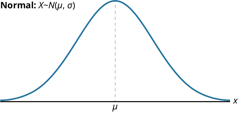
A symmetrical, bell-shaped curve is centered around the mean (µ) on the x-axis. The equation “X~N(µ, s)” signifies that X follows this distribution with mean µ and standard deviation s. The dashed line intersects the curve’s peak at the mean. — **Figure 3.7** Graph of the Normal (Bell-Shaped) Distribution

The curve in Figure 3.7 is symmetric on either side of a vertical line drawn through the mean, $µ$ . The mean is the same as the median, which is the same as the mode, because the graph is symmetric about $µ$ . As the notation indicates, the normal distribution depends only on the mean and the standard deviation. Because the area under the curve must equal 1, a change in the standard deviation, $σ$ , causes a change in the shape of the normal curve; the curve becomes fatter and wider or skinnier and taller depending on $σ$ . A change in $µ$ causes the graph to shift to the left or right. This means there are an infinite number of normal probability distributions.

To determine probabilities associated with the normal distribution, we find specific areas under the normal curve. There are several methods for finding this area under the normal curve, and we typically use some form of technology. Python, Excel, and R all provide built-in functions for calculating areas under the normal curve.

Example 6

Suppose that at a software company, the mean employee salary is $60,000 with a standard deviation of $7,500. Assume salaries at this company follow a normal distribution. Use Python to calculate the probability that a random employee earns more than $68,000.

A normal curve can be drawn to represent this scenario, in which the mean of $60,000 would be plotted on the horizontal axis, corresponding to the peak of the curve. Then, to find the probability that an employee earns more than $68,000, calculate the area under the normal curve to the right of the data value $68,000.

Figure 3.8 illustrates the area under the normal curve to the right of a salary of $68,000 as the shaded-in region.

Figure 3.8 Bell-Shaped Distribution for Example 6. The shaded region under the normal curve corresponds to the probability that an employee earns more than $68,000.

To find the actual area under the curve, a Python command can be used to find the area under the normal probability density curve to the right of the data value of $68,000. See Using Python with Probability Distributions for the specific Python program and results. The resulting probability is calculated as 0.143.

Thus, there is a probability of about 14% that a random employee has a salary greater than $75,000.

The empirical rule is a method for determining approximate areas under the normal curve for measurements that fall within one, two, and three standard deviations from the mean for the normal (bell-shaped) distribution. (See Figure 3.9).

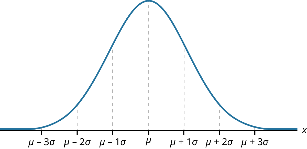
A symmetric, bell-shaped curve is centered around the mean (µ), with values from -3s to +3s on the x-axis. Data clusters around the mean, with observations decreasing in both directions as they move away. The peak at µ is the most common value; the tails capture extreme values. — **Figure 3.9** Normal Distribution Showing Mean and Increments of Standard Deviation

If $x$ is a continuous random variable and has a normal distribution with mean $µ$ and standard deviation $σ$ , then the empirical rule states that:

About 68% of the $x$ -values lie between $minus 1 σ$ and $plus 1 σ$ units from the mean $µ$ (within one standard deviation of the mean).
About 95% of the $x$ -values lie between $minus 2 σ$ and $plus 2 σ$ units from the mean $µ$ (within two standard deviations of the mean).
About 99.7% of the $x$ -values lie between $minus 3 σ$ and $plus 3 σ$ units from the mean $µ$ (within three standard deviations of the mean). Notice that almost all the x-values lie within three standard deviations of the mean.
The $z$ -scores for $plus 1 σ$ and $minus 1 σ$ are $plus 1$ and $minus 1$ , respectively.
The $z$ -scores for $plus 2 σ$ and $minus 2 σ$ are $plus 2$ and $minus 2$ , respectively.
The $z$ -scores for $plus 3 σ$ and $minus 3 σ$ are $plus 3$ and $minus 3$ , respectively.

Example 7

An automotive designer is interested in designing automotive seats to accommodate the heights for about 95% of customers. Assume the heights of adults follow a normal distribution with mean of 68 inches and standard deviation of 3 inches. For what range of heights should the designer model the car seats to accommodate 95% of drivers?

According to the empirical rule, the area under the normal curve within two standard deviations of the mean is 95%. Thus, the designer should design the seats to accommodate heights that are two standard deviations away from the mean. The lower bound of heights would be $68 minus 2 open parenthesis 3 close parenthesis$ inches, and the upper bound of heights would be $68 plus 2 open parenthesis 3 close parenthesis$ inches. Thus, the car seats should be designed to accommodate driver heights between 62 and 74 inches.

Using Python with Probability Distributions

Python provides a number of built-in functions for calculating probabilities associated with both discrete and continuous probability distributions such as binomial distribution and the normal distribution. These functions are part of a library called scipy.stats.

Here are a few of these probability density functions available within Python:

binom—calculate probabilities associated with the binomial distribution
poisson—calculate probabilities associated with the Poisson distribution
expon—calculate probabilities associated with the exponential distribution
norm—calculate probabilities associated with the normal distribution

To import these probability density functions within Python, use the import command. For example, to import the binom function use the following command:
from scipy.stats import binom

Using Python with the Binomial Distribution

The binom function in Python allows calculations of binomial probabilities. The probability mass function for the binomial distribution within Python is referred to as binom.pmf.

The syntax for using this function is binom.pmf(x, n, p)

Where:
$n$ is the number of trials in the experiment
$p$ is the probability of success
$x$ is the number of successes in the experiment

Consider the previous Example 3 worked out using the Python binom.pmf function. A medical researcher is conducting a study related to a certain type of shoulder surgery. A sample of 20 patients who have recently undergone the surgery is selected, and the researcher wants to determine the probability that 18 of the 20 patients had a successful result from the surgery. From past data, the researcher knows that the probability of success for this type of surgery is 92%. Round your answer to 3 decimal places.

In this example:
$n$ is the number of trials in the experiment $equals 20$
$p$ is the probability of success $equals 0.92$
$x$ is the number of successes in the experiment $equals 18$

The corresponding function in Python is written as:

binom.pmf (18, 20, 0.92)

The round function is then used to round the probability result to 3 decimal places.

Here is the input and output of this Python program:

Note

# import the binom function from the scipy.stats library
from scipy.stats import binom

# define parameters x, n, and p:
x = 18
n = 20
p = 0.92

# use binom.pmf() function to calculate binomial probability
# use round() function to round answer to 3 decimal places
round (binom.pmf(x, n, p), 3)

The resulting output will look like this:

0.271

Using Python with the Normal Distribution

The norm function in Python allows calculations of normal probabilities. The probability density function is sometimes called the cumulative density function, and so this is referred to as norm.cdf within Python. The norm.cdf function returns the area under the normal probability density function to the left of a specified measurement.

The syntax for using this function is
norm.cdf(x, mean, standard_deviation)

Where:
x is the measurement of interest
mean is the mean of the normal distribution
standard_deviation is the standard deviation of the normal distribution

Let’s work out the previous Example 6 using the Python norm.cdf function.

Suppose that at a software company, the mean employee salary is $60,000 with a standard deviation of $7,500. Use Python to calculate the probability that a random employee earns more than $68,000.

In this example:
$x$ is the measurement of interest $equals 68,000$
mean is the mean of the normal distribution $equals 60,000$
standard deviation is the standard deviation of the normal distribution $equals 7,500$

The corresponding function in Python is written as:
norm.cdf(68000, 60000, 7500)

The round function is then used to round the probability result to 3 decimal places.

Notice that since this example asks to find the area to the right of a salary of $68,000, we can first find the area to the left using the norm.cdf function and subtract this area from 1 to then calculate the desired area to the right.

Here is the input and output of the Python program:

Note

# import the norm function from the scipy.stats library
from scipy.stats import norm
# define parameters x, mean and standard_deviation:
x = 68000
mean = 60000
standard_deviation = 7500
# use norm.cdf() function to calculate normal probability - note this is
# the area to the left
# subtract this result from 1 to obtain area to the right of the x-value
# use round() function to round answer to 3 decimal places
round (1 - norm.cdf(x, mean, standard_deviation), 3)

The resulting output will look like this:

0.143

Analysis of Salary Data by Gender

There are many sources of salary data where median salaries for a certain year are published by gender. One source for data on earnings by demographics is the Bureau of Labor Statistics.

As a group:

Research salary data by gender for a certain year.
Compile descriptive statistics where available for statistical measurements including the mean, median, quartiles, and standard deviation by gender.
Create graphical presentations for this data using histograms, side-by-side box plots, and time series graphs.
Discuss the following:
1. From your analysis, does there appear to be a wage gap for men’s vs. women’s salaries?
2. If so, is the wage gap improving over time or worsening over time?