
3.3 Measures of Position
Learning Outcomes
By the end of this section, you should be able to:
- Define and calculate percentiles, quartiles, and -scores for a dataset.
- Use Python to calculate measures of position for a dataset.
Common measures of position include percentiles and quartiles as well as -scores, all of which are used to indicate the relative location of a particular datapoint.
Percentiles
If a student scores 47 on a biology exam, it is difficult to know if the student did well or poorly compared to the population of all other students taking the exam. Percentiles provide a way to assess and compare the distribution of values and the position of a specific data point in relation to the entire dataset by indicating the percentage of data points that fall below it. Specifically, a percentile is a value on a scale of one hundred that indicates the percentage of a distribution that is equal to or below it. Let’s say the student learns they scored in the 90th percentile on the biology exam. This percentile indicates that the student has an exam score higher than 90% of all other students taking the test. This is the same as saying that the student’s score places the student in the top 10% of all students taking the biology test. Thus, this student scoring in the 90th percentile did very well on the exam, even if the actual score was 47.
To calculate percentiles, the data must be ordered from smallest to largest and then the ordered data divided into hundredths. If you score in the 80th percentile on an aptitude test, that does not necessarily mean that you scored 80% on the test. It means that 80% of the test scores are the same as or less than your score and the remaining 20% of the scores are the same as or greater than your score.
Percentiles are useful for comparing many types of values. For example, a stock market mutual fund might report that the performance for the fund over the past year was in the 80th percentile of all mutual funds in the peer group. This indicates that the fund performed better than 80% of all other funds in the peer group. This also indicates that 20% of the funds performed better than this particular fund.
To calculate percentiles for a specific data value in a dataset, first order the dataset from smallest to largest and count the number of data values in the dataset. Locate the measurement of interest and count how many data values fall below the measurement. Then the percentile for the measurement is calculated as follows:
Quartiles
While percentiles separate data into 100 equal parts, quartiles separate data into quarters, or four equal parts. To find the quartiles, first find the median, or second quartile. The first quartile, , is the middle value, or median, of the lower half of the data, and the third quartile, , is the middle value of the upper half of the data.
Note the following correspondence between quartiles and percentiles:
- The first quartile corresponds to the 25th percentile.
- The second quartile (which is the median) corresponds to the 50th percentile.
- The third quartile corresponds to the 75th percentile.
The interquartile range (IQR) is a number that indicates the spread of the middle half, or the middle 50%, of the data. It is the difference between the third quartile, , and the first quartile, .
Note that the IQR provides a measure of variability that excludes outliers.
In Example 2, the IQR can be calculated as:
Quartiles and the IQR can be used to flag possible outliers in a dataset. For example, if most employees at a company earn about $50,000 and the CEO of the company earns $2.5 million, then we consider the CEO’s salary to be an outlier data value because this salary is significantly different from all the other salaries in the dataset. An outlier data value can also be a value much lower than the other data values in a dataset, so if one employee only makes $15,000, then this employee’s low salary might also be considered an outlier.
To detect outliers, you can use the quartiles and the IQR to calculate a lower and an upper bound for outliers. Then any data values below the lower bound or above the upper bound will be flagged as outliers. These data values should be further investigated to determine the nature of the outlier condition and whether the data values are valid or not.
To calculate the lower and upper bounds for outliers, use the following formulas:
These formulas typically use 1.5 as a cutoff value to identify outliers in a dataset.
-scores
The -score is a measure of the position of an entry in a dataset that makes use of the mean and standard deviation of the data. It represents the number of standard deviations by which a data value differs from the mean. For example, suppose that in a certain neighborhood, the mean selling price of a home is $350,000 and the standard deviation is $40,000. A particular home sells for $270,000. Based on the selling price of this home, we can calculate the relative standing of this home compared to other home sales in the same neighborhood.
The corresponding -score of a measurement considers the given measurement in relation to the mean and standard deviation for the entire population. The formula for a -score calculation is as follows:
Where:
is the measurement
is the mean
is the standard deviation
Notice that when a measurement is below the mean, the corresponding -score will be a negative value. If the measurement is exactly equal to the mean, the corresponding -score will be zero. If the measurement is above the mean, the corresponding -score will be a positive value.
-scores can also be used to identify outliers. Since -scores measure the number of standard deviations from the mean for a data value, a -score of 3 would indicate a data value that is 3 standard deviations above the mean. This would represent a data value that is significantly displaced from the mean, and typically, a -score less than −3 or a -score greater than +3 can be used to flag outliers.
Using Python to Calculate Measures of Position for a Dataset
DataFrame.describe computes different measures of position as well on each column of a dataset. See min, 25%, 50%, 75%, and max in Figure 3.4.
import pandas as pd

movies = pd.read_csv("ch1-movieprofit.csv")
print("rows:", len(movies))
print(movies.describe().round(2).to_string())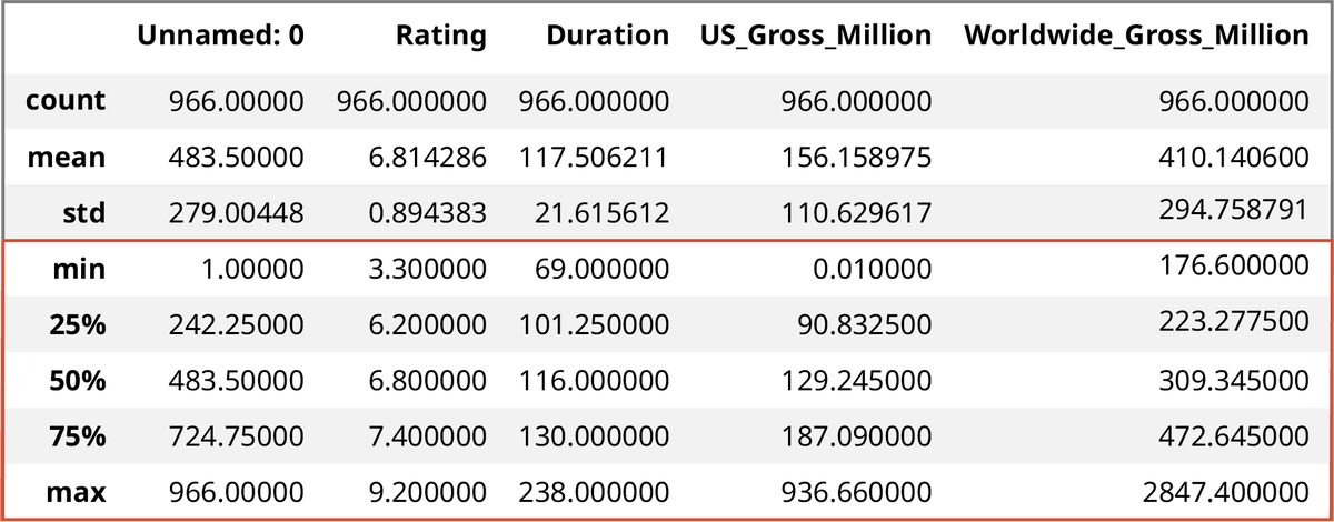
DataFrame.describe with the Movie Profit DatasetAdapted from Principles of Data Science by OpenStax (openstax.org), licensed under CC BY-NC-SA 4.0. Changes were made. License: CC-BY-NC-SA-4.0.