
1.3 Data and Datasets
Learning Outcomes
By the end of this section, you should be able to:
- Define data and dataset.
- Differentiate among the various data types used in data science.
- Identify the type of data used in a dataset.
- Discuss an item and attribute of a dataset.
- Identify the different data formats and structures used in data science.
What Is Data Science? and Data Science in Practice introduced the many varieties of and uses for data science in today’s world. Data science allows us to extract insights and knowledge from data, driving decision-making and innovation in business, health care, entertainment, and so on. As we’ve seen, the field has roots in math, statistics, and computer science, but it only began to emerge as its own distinct field in the early 2000s with the proliferation of digital data and advances in computing power and technology. It gained significant momentum and recognition around the mid to late 2000s with the rise of big data and the need for sophisticated techniques to analyze and derive insights from large and complex datasets. Its evolution since then has been rapid, and as we can see from the previous discussion, it is quickly becoming a cornerstone of many industries and domains.
Data, however, is not new! Humans have been collecting data and generating datasets from the beginning of time. This started in the Stone Age when people carved some shapes and pictures, called petroglyphs, on rock. The petroglyphs provide insights on how animals looked and how they carried out their daily life, which is valuable “data” for us. Ancient Egyptians invented a first form of paper—papyrus—in order to journal their data. Papyrus also made it easier to store data in bulk, such as listing inventories, noting financial transactions, and recording a story for future generations.
Data
“Data” is the plural of the Latin word “datum,” which translates as something that is given or used and is often used to mean a single piece of information or a single point of reference in a dataset. When you hear the word “data,” you may think of some sort of “numbers.” It is true that numbers are usually considered data, but there are many other forms of data all around us. Anything that we can analyze to compile information—high-level insights—is considered data.
Suppose you are debating whether to take a certain course next semester. What process do you go through in order to make your decision? First, you might check the course evaluations, as shown in Table 1.1.
| Semester | Instructor | Class Size | Rating |
|---|---|---|---|
| Fall 2020 | A | 100 | Not recommended at all |
| Spring 2021 | A | 50 | Highly recommended |
| Fall 2021 | B | 120 | Not quite recommended |
| Spring 2022 | B | 40 | Highly recommended |
| Fall 2022 | A | 110 | Recommended |
| Spring 2023 | B | 50 | Highly recommended |
The evaluation record consists of four kinds of data, and they are grouped as columns of the table: Semester, Instructor, Class Size, and Rating. Within each column there are six different pieces of data, located at each row. For example, there are six pieces of text data under the Semester column: “Fall 2020,” “Spring 2021,” “Fall 2021,” “Spring 2022,” “Fall 2022,” and “Spring 2023.”
The course evaluation ratings themselves do not provide an idea on whether to take the course next semester. The ratings are just a phrase (e.g., “Highly recommended” or “Not quite recommended”) that encodes how recommended the course was in that semester. You need to analyze them to come up with a decision!
Now let’s think about how to derive the information from these ratings. You would probably look at all the data, including when in the semester the course was offered, who the instructor is, and class size. These records would allow you to derive information that would help you decide “whether or not to take the course next semester.”
Types of Data
The previous sections talked about how much our daily life is surrounded by data, how much our daily life itself produces new data, and how often we make data-driven decisions without even noticing it. You might have noticed that data comes in various types. Some data are quantitative, which means that they are measured and expressed using numbers. Quantitative data deals with quantities and amounts and is usually analyzed using statistical methods. Examples include numerical measurements like height, weight, temperature, heart rate, and sales figures. Qualitative data are non-numerical data that generally describe subjective attributes or characteristics and are analyzed using methods such as thematic analysis or content analysis. Examples include descriptions, observations, interviews, and open-ended survey responses (as we’ll see in Survey Design and Implementation) that address unquantifiable details (e.g., photos, posts on Reddit). The data types often dictate methods for data analysis, so it is important to be able to identify a type of data. Thus, this section will take a further dive into types of data.
Let’s revisit our previous example about deciding whether to take a certain course next semester. In that example, we referred to four pieces of data. They are encoded in different types such as numbers, words, and symbols.
- The semester the course was offered—Fall 2020, Spring 2021, …, Fall 2022, Spring 2023
- The instructor—A and B
- The class size—100, 50, 120, 40, 110, 50
- The course rating—“Not recommended at all,” …, “Highly recommended”
There are two primary types of quantitative data—numeric and categorical—and each of these can be divided into a few subtypes. Numeric data is represented in numbers that indicate measurable quantities. It may be followed by some symbols to indicate units. Numeric data is further divided into continuous data and discrete data. With continuous data, the values can be any number. In other words, a value is chosen from an infinite set of numbers. With discrete data, the values follow a specific precision, which makes the set of possible values finite.
From the previous example, the class size 100, 150, etc. are numbers with the implied unit “students.” Also, they indicate measurable quantities as they are head counts. Therefore, the class size is numeric data. It is also continuous data since the size numbers seem to be any natural numbers and these numbers are chosen from an infinite set of numbers, the set of natural numbers. Note that whether data is continuous (or discrete) also depends on the context. For example, the same class size data can be discrete if the campus enforces all classes to be 200 seats or less. Such restriction makes the class size values be chosen from a finite set of 200 numbers: 1, 2, 3, …, 198, 199, 200.
Categorical data is represented in different forms such as words, symbols, and even numbers. A categorical value is chosen from a finite set of values, and the value does not necessarily indicate a measurable quantity. Categorical data can be divided into nominal data and ordinal data. For nominal data, the set of possible values does not include any ordering notion, whereas with ordinal data, the set of possible values includes an ordering notion.
The rest—semester, instructor, and ratings—are categorical data. They are represented in symbols (e.g., “Fall 2020,” “A”) or words (e.g., “Highly recommended”), and these values are chosen from the finite set of those symbols and words (e.g., A vs. B). The former two data are nominal since the semester and instructor do not have orders to follow, while the latter is ordinal since there is a notion of degree (Not recommended at all ~ Highly recommended). You may argue that the semester could have chronological ordering: Fall 2020 comes before Spring 2021, Fall 2021 follows Fall 2020. If you want to value that notion for your analysis, you could consider the semester data to be ordinal as well—the chronological ordering is indeed critical when you are looking at a time-series dataset. You will learn more about that in Time Series and Forecasting.
Datasets
A dataset is a collection of observations or data entities organized for analysis and interpretation, as shown in Table 1.1. Many datasets can be represented as a table where each row indicates a unique data entity and each column defines the structure of the entities.
Notice that the dataset we used in Table 1.1 has six entities (also referred to as items, entries, or instances), distinguished by semester. Each entity is defined by a combination of four attributes or characteristics (also known as features or variables)—Semester, Instructor, Class Size, and Rating. A combination of features characterizes an entry of a dataset.
Although the actual values of the attributes are different across entities, note that all entities have values for the same four attributes, which makes them a structured dataset. As a structured dataset, these items can be listed as a table where each item is listed along the rows of the table.
By contrast, an unstructured dataset is one that lacks a predefined or organized data model. While structured datasets are organized in a tabular format with clearly defined fields and relationships, unstructured data lacks a fixed schema. Unstructured data is often in the form of text, images, videos, audio recordings, or other content where the information doesn't fit neatly into rows and columns.
There are plenty of unstructured datasets. Indeed, some people argue there are more unstructured datasets than structured ones. A few examples include Amazon reviews on a set of products, Twitter posts last year, public images on Instagram, popular short videos on TikTok, etc. These unstructured datasets are often processed into a structured one so that data scientists can analyze the data. We’ll discuss different data processing techniques in Collecting and Preparing Data.
Dataset Formats and Structures (CSV, JSON, XML)
Datasets can be stored in different formats, and it’s important to be able to recognize the most commonly used formats. This section covers three of the most often used formats for structured datasets—comma-separated values (CSV), JavaScript Object Notation (JSON), and Extensible Markup Language (XML). While CSV is the most intuitive way of encoding a tabular dataset, much of the data we would collect from the web (e.g., websites, mobile applications) is stored in the JSON or XML format. The reason is that JSON is the most suitable for exchanging data between a user and a server, and XML is the most suitable for complex dataset due to its hierarchy-friendly nature. Since they all store data as plain texts, you can open them using any typical text editors such as Notepad, Visual Studio Code, Sublime Text, or VI editor.
Table 1.3 summarizes the advantages and disadvantages of CSV, JSON, and XML dataset formats. Each of these is described in more detail below.
| Dataset Format | Pros | Cons | Typical Use |
|---|---|---|---|
| CSV | Simple | Difficult to add metadata Difficult to parse if there are special characters Flat structure | Tabular data |
| JSON | Simple Compatible with many languages Easy to parse | Difficult to add metadata Cannot leave comments | Data that needs to be exchanged between a user and a server |
| XML | Structured (so more readable) Possible to add metadata | Verbose Complex structure with tags | Hierarchical data structures |
Comma-Separated Values (CSV)
The CSV stores each item in the dataset in a single line. Variable values for each item are listed all in one line, separated by commas (“,”). The previous example about signing up for a course can be stored as a CSV file. Figure 1.4 shows how the dataset looks when opened with a text editor (e.g., Notepad, TextEdit, MS Word, Google Doc) or programming software in the form of a code editor (e.g., Sublime Text, Visual Studio Code, XCode). Notice that commas are used to separate the attribute values within a single line (see Figure 1.4).
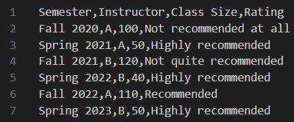
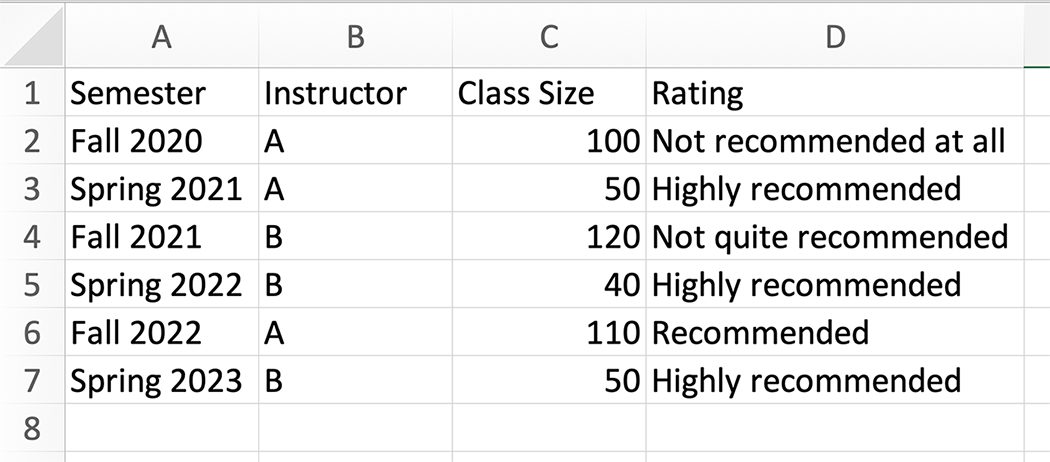
CSV files can be opened with spreadsheet software such as MS Excel and Google Sheets. The spreadsheet software visualizes CSV files more intuitively in the form of a table (see Figure 1.5). We will cover the basic use of Python for analyzing CSV files in Data Science with Python.
JavaScript Object Notation (JSON)
JSON uses the syntax of a programming language named JavaScript. Specifically, it follows JavaScript’s object syntax. Don’t worry, though! You do not need to know JavaScript to understand the JSON format.
Figure 1.7 provides an example of the JSON representation of the same dataset depicted in Figure 1.6.

Notice that the JSON format starts and ends with a pair of curly braces ({}). Inside, there are multiple pairs of two fields that are separated by a colon (:). These two fields that are placed on the left and right of the colon are called a key and value, respectively,—key: value. For example, the dataset in Figure 1.7 has five pairs of key-values with the key "Semester": "Fall 2020", "Semester": "Spring 2021", "Semester": "Fall 2021", "Semester": "Spring 2022", "Semester": "Fall 2022", and "Semester": "Spring 2023".
CourseEvaluations.json has one key-value pair at the highest level: "Members": [...]. You can see that each item of the dataset is listed in the form of an array or list under the key "Members". Inside the array, each item is also bound by curly braces and has a list of key-value pairs, separated by commas. Keys are used to describe attributes in the dataset, and values are used to define the corresponding values. For example, the first item in the JSON dataset above has four keys, each of which maps to each attribute—Semester, Instructor, Class Size, and Rating. Their values are "Fall 2020", "A", 100, and "Not recommended at all".
Extensible Markup Language (XML)
The XML format is like JSON, but it lists each item of the dataset using different symbols named tags. An XML tag is any block of text that consists of a pair of angle brackets (< >) with some text inside. Let’s look at the example XML representation of the same dataset in Figure 1.8. Note that the screenshot of CourseEvaluations.xml below only includes the first three items in the original dataset.
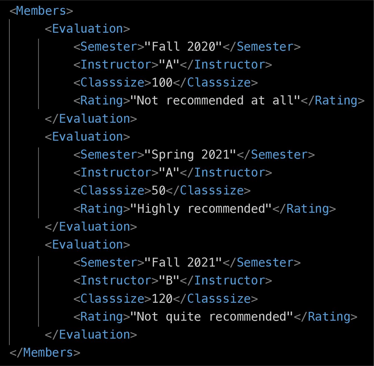
CourseEvaluations.xml lists each item of the dataset between a pair of tags, <members> and </members>. Under <members>, each item is defined between <evaluation> and </evaluation>. Since the dataset in Figure 1.8 has three items, we can see three blocks of <evaluation>... </evaluation>. Each item has four attributes, and they are defined as different XML tags as well—<semester>, <instructor>, <classsize>, and <rating>. They are also followed by closing tags such as </semester>, </instructor>, </classsize>, and </rating>.
PubMed datasets provides a list of articles that are published in the National Library of Medicine in XML format. Click Annual Baseline and download/open any.xml file. Note that all the.xml files are so big that they are compressed to.gz files. However, once you download one and attempt to open it by double-clicking, the file will automatically be decompressed and open. You will see a bunch of XML tags along with information about numerous publications, such as published venue, title, published date, etc.
XML and Image Data
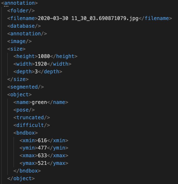
The XML format is also commonly used as an attachment to some image data. It is used to note supplementary information about the image. For example, the Small Traffic Light Dataset in Figure 1.9 comes with a set of traffic light images, placed in one of the three directories: JPEGImages, train_images, and valid_images. Each image directory is accompanied with another directory just for annotations such as Annotations, train_annotations, and valid_annotations.
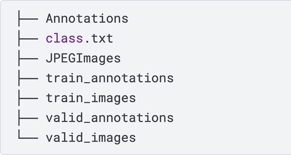
The annotation directories have a list of XML files, each of which corresponds to an image file with the same filename inside the corresponding image directory (Figure 1.10). Figure 1.11 shows that the first XML file in the Annotations directory includes information about the.jpg file with the same filename.
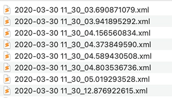
(source: “Small Traffic Light Dataset,” https://www.kaggle.com/datasets/sovitrath/small-traffic-light-dataset-xml-format)
JSON and XML Dataset Descriptions
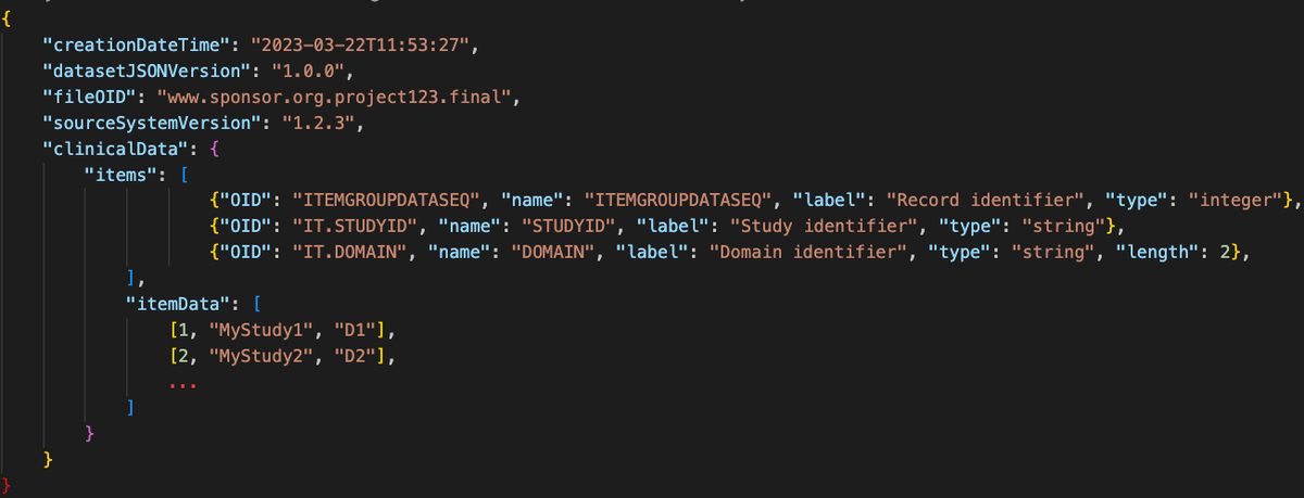
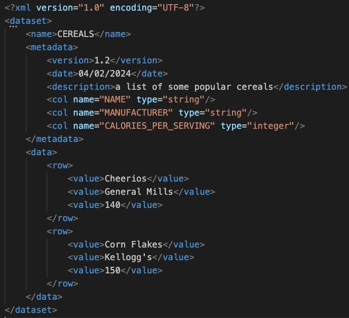
Both JSON and XML files often include some description(s) of the dataset itself as well (known as metadata), and they are included as a separate entry in the file ({} or <>). In Figure 1.12 and Figure 1.13, the actual data entries are listed inside “itemData” and <data>, respectively. The rest are used to provide background information on the dataset. For example:
- “creationDateTime”: describes when the dataset was created.
<name>is used to write the name of this dataset.<metadata>is used to describe each column name of the dataset along with its data type.
The Face Mask Detection dataset has a set of images of human faces with masks on. It follows a similar structure as well. The dataset consists of two directories—annotations and images. The former is in the XML format. The name of each XML file includes any text description about the image with the same filename. For example, “maksssksksss0.xml” includes information on “maksssksksss0.png.”
Adapted from Principles of Data Science by OpenStax (openstax.org), licensed under CC BY-NC-SA 4.0. Changes were made. License: CC-BY-NC-SA-4.0.