9.8 Sampling Distribution of p

Assume that in an election race between Candidate A and Candidate B, 0.60 of the voters prefer Candidate A. If a random sample of 10 voters were polled, it is unlikely that exactly 60% of them (6) would prefer Candidate A. By chance the proportion in the sample preferring Candidate A could easily be a little lower than 0.60 or a little higher than 0.60. The sampling distribution of p is the distribution that would result if you repeatedly sampled 10 voters and determined the proportion (p) that favored Candidate A.

The sampling distribution of p is a special case of the sampling distribution of the mean. Table 1 shows a hypothetical random sample of 10 voters. Those who prefer Candidate A are given scores of 1 and those who prefer Candidate B are given scores of 0. Note that seven of the voters prefer candidate A so the sample proportion (p) is

p = 7/10 = 0.70

As you can see, p is the mean of the 10 preference scores.

Table 1. Sample of voters.

Voter	Preference
1	1
2	0
3	1
4	1
5	1
6	0
7	1
8	0
9	1
10	1

The distribution of p is closely related to the binomial distribution. The binomial distribution is the distribution of the total number of successes (favoring Candidate A, for example) whereas the distribution of p is the distribution of the mean number of successes. The mean, of course, is the total divided by the sample size, N. Therefore, the sampling distribution of p and the binomial distribution differ in that p is the mean of the scores (0.70) and the binomial distribution is dealing with the total number of successes (7).

The binomial distribution has a mean of

μ = Nπ

Dividing by N to adjust for the fact that the sampling distribution of p is dealing with means instead of totals, we find that the mean of the sampling distribution of p is:

μ_p = π

The standard deviation of the binomial distribution is:

$\sqrt{N π (1 - π)}$

Dividing by N because p is a mean not a total, we find the standard error of p:

$σ_{p} = \frac{\sqrt{N π (1 - π)}}{N} = \sqrt{\frac{π (1 - π)}{N}}$

Returning to the voter example, π = 0.60 and N = 10. (Don't confuse π = 0.60, the population proportion and p = 0.70, the sample proportion.) Therefore, the mean of the sampling distribution of p is 0.60. The standard error is

$σ_{p} = \sqrt{\frac{0.60 (1 - .60)}{10}} = 0.155$

The sampling distribution of p is a discrete rather than a continuous distribution. For example, with an N of 10, it is possible to have a p of 0.50 or a p of 0.60 but not a p of 0.55.

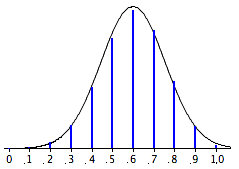
The sampling distribution of p is approximately normally distributed if N is fairly large and π is not close to 0 or 1. A rule of thumb is that the approximation is good if both Nπ and N(1 - π) are greater than 10. The sampling distribution for the voter example is shown in Figure 1. Note that even though N(1 - π) is only 4, the approximation is quite good.

The sampling distribution of the sample proportion p for N = 10 and a population proportion of 0.60, drawn as blue vertical spikes at 0, .1, .2, ... 1.0 with a smooth normal curve laid over them. The spikes are tallest at .6, then .5 and .7, and the curve passes close to the top of each — the normal approximation is good here even though N(1 - pi) is only 4. — Figure 1. The sampling distribution of p. Vertical bars are the probabilities; the smooth curve is the normal approximation.

Adapted from Online Statistics Education: A Multimedia Course of Study (onlinestatbook.com), Project Leader: David M. Lane, Rice University. Developed with NSF support. The original work is in the public domain; it is cited here at the authors' request. Changes were made: reformatted as an accessible XYZ web edition with native MathML. License: Public-Domain.