
5.8 Binomial Demonstration
This section is an interactive demonstration. The live simulation runs on the original site: open the demonstration at onlinestatbook.com.
Learning Objectives
- State the relationship beween p and skew.
- Compute the mean and standard deviation of a binomial distribution
- State how N affects the shape of a binomial distribution.
Instructions
This demonstration allows you to explore the binomial distribution. Here you can specify the number of trials (N) and the propotion of successes (p). Note that the proporton of successes is sometimes referred to with the Greek letter p; here it will be referred to as p.
The starting values for N and p are 10 and 0.5. The graph therefore shows the probability of from 0 to 10 successes out of 10 trials. The probability of 0 successes is so small that it just barely shows up on the graph. The most likely number of successes is 5, which has a probability of about 0.25. Naturally, the sum of the probabilities is 1.0.
The demonstration also shows the mean and the standard deviation of the binomial distribution.
Illustrated Instructions
The screenshot below shows the binomial demonstration with its default data. You can adjust the
number of trials (N) as well as the proportion of successes (p).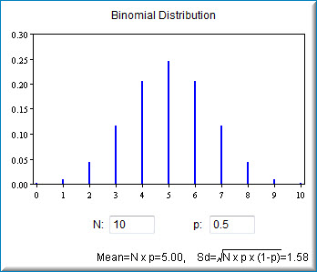
The example below shows a distribution of 20 trials with a probability of success of .7. Notice that the mean and standard deviation for the distribution are also shown.
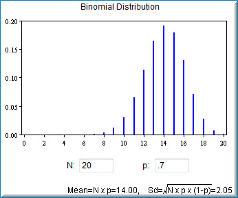
The graph will adjust to the entered number of trials (N) and probability of success (P).
Adapted from Online Statistics Education: A Multimedia Course of Study (onlinestatbook.com), Project Leader: David M. Lane, Rice University. Developed with NSF support. The original work is in the public domain; it is cited here at the authors' request. Changes were made: reformatted as an accessible XYZ web edition with native MathML. License: Public-Domain.