4.3 Lagrange Multipliers

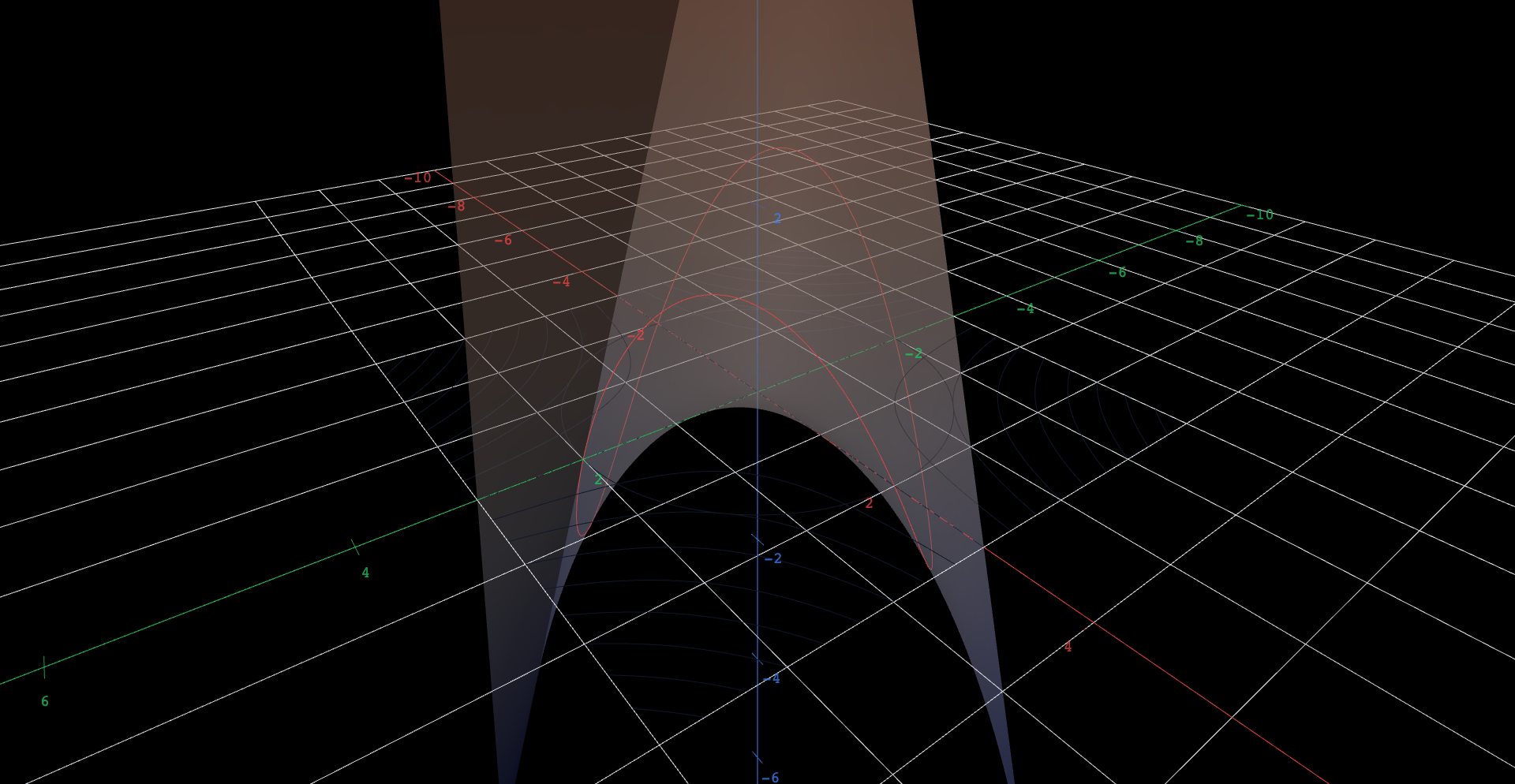
Most optimization in practice comes with a leash: maximize $f$ , subject to $g = c$ . The leash changes everything. A constrained maximum is almost never at a critical point of $f$ itself — our specimen $f (x, y) = x y$ has only a saddle, no maximum at all — yet on the constraint circle $x^{2} + y^{2} = 4$ the problem has clean, finite answers. The question is where to look, and the figure answers it twice over: once on the map, once along a ribbon.

A translucent red-and-blue saddle surface z = x*y with seventeen dark contour lines on the z = 0 plane — hyperbolas, plus a crossed pair of straight lines at level zero. A flat dark circle of radius 2 lies in that plane, and a thick red ribbon-like curve traces the value of x*y above and below each point of the circle, rising to two crests of height 2 and dipping to two troughs of depth 2. Two red marker points at the crests are hidden. — The translucent red-and-blue saddle $z = x y$ , its seventeen dark level curves on the plane $z equals 0$ (hyperbolas, plus a crossed pair of lines at level $0$ ), a flat dark circle of radius $2$ in that same plane — the constraint $x^{2} + y^{2} = 4$ — and a thick red ribbon that follows the circle while rising and falling with the surface: $f$ evaluated along the constraint, the only part of the surface the problem is allowed to use. Two marker points at the constrained maxima hide in the object list.

Explore

Orbit to a low side view and follow the red ribbon once around. How many crests and how many troughs does it have? Note roughly where the crests sit over the dark circle.
A crest is where $f$ , walking along the constraint, stops increasing and starts decreasing — it stalls. What is the ribbon's slope, measured along the walk, at a stall?
The ribbon's height over the circle is $x y$ . Using symmetry — the product is largest where $x$ and $y$ are equal and share a sign — predict the exact coordinates of the two crests and the value of $f$ there. Commit before revealing.
Reveal the two hidden points with their eye toggles. They sit at the crests; zoom in and read their positions against the grid. Do they match your $(\pm \sqrt{2}, \pm \sqrt{2})$ , $f equals 2$ ?
Now the map view: orbit to look straight down and drag the contour plot's z-offset from $0$ up to $2$ . The whole family of level curves rides up the saddle as one sheet. As it reaches crest height, the curve $x y equals 2$ meets the circle at exactly the two marked points — does it cross the circle there, or kiss it tangentially?
Drag the z-offset back to about $1$ and look at where $x y equals 1$ meets the circle: four honest crossings. Check against the ribbon — over those four points, is it at a crest, or still climbing? Say the connection out loud: crossing a level curve means the walk is still changing $f$ . (The 17 levels put drawn curves exactly at the integer values $minus 8, …, 8$ , so both curves in this step and the last are actually drawn; other level counts can hide them.)

From kiss to equations

At a tangency the constraint curve and the level curve share a tangent line, so their normals point along one line. Those normals are gradients — $∇ f$ for the level curve, $∇ g$ for the constraint — so at a constrained extremum

$∇ f equals λ ∇ g$

for some scalar $λ$ , the Lagrange multiplier, solved together with $g = c$ . The logic runs through step 6: where the level curve crosses the constraint, level curves of larger and smaller value lie on either side, so sliding along the constraint still changes $f$ — no extremum there. Only a kiss can stop the walk, and the ribbon says the same thing in its own language: kisses on the map are stalls on the ribbon.

Example 1 The full Lagrange computation on the circle

Find the maximum and minimum of $f (x, y) = x y$ on the circle $x^{2} + y^{2} = 4$ , with the multiplier at each.

With $g = x^{2} + y^{2}$ , the equations $∇ f equals λ ∇ g$ and the constraint read

$y = 2 λ x, x = 2 λ y, x^{2} + y^{2} = 4 .$

Substituting the first into the second gives $x equals 4 λ squared x$ . If $x equals 0$ the first equation forces $y equals 0$ , violating the constraint — so $λ^{2} = \frac{1}{4}$ , i.e. $λ = \pm \frac{1}{2}$ . For $λ = \frac{1}{2}$ the equations give $y = x$ , and the constraint gives $2 x squared equals 4$ : the points $(\sqrt{2}, \sqrt{2})$ and $(- \sqrt{2}, - \sqrt{2})$ , where $f equals 2$ . For $λ = - \frac{1}{2}$ , $y = - x$ yields $(\sqrt{2}, - \sqrt{2})$ and $(- \sqrt{2}, \sqrt{2})$ , where $f = - 2$ . So the constrained maximum is $2$ and the minimum $minus 2$ . The ribbon confirms it in one variable: on the circle, $f (2 \cos t, 2 \sin t) = 4 \cos t \sin t = 2 \sin 2 t$ , which crests at $2$ and bottoms at $minus 2$ , four stalls per lap — exactly the four kisses.

\frac{1}{2}, - \frac{1}{2}

The multiplier equation, solved ✓ Computed · mojocas 0.1.0 ✓ Agrees with the text

The pivot of the example: eliminating $x$ and $y$ from the Lagrange equations leaves $4 λ squared equals 1$ (written here with $L$ for $λ$ ), whose two roots $λ = \pm \frac{1}{2}$ hand back the lines $y = x$ and $y = - x$ and, with the constraint, all four kiss points.

An original work of XYZ Homework, built around interactive XYZ 3D figures. Aligned to OpenStax Calculus Volume 3 (Strang & Herman), © OpenStax (Rice University), licensed CC BY-NC-SA 4.0; no OpenStax content is reproduced, and this work is not affiliated with or endorsed by OpenStax or Rice University. License: CC-BY-NC-SA-4.0.