4.1 Linear Phase Portraits

The simplest system of two equations is one whose equations ignore each other:

$x' = x, \qquad y' = -y.$

Each unknown solves on its own: $x(t) = x_0 e^{t}$ grows, $y(t) = y_0 e^{-t}$ decays. The two rates, $+1$ and $-1$ , are the system's eigenvalues, and the directions along which the motion is pure exponential growth or pure exponential decay — here, the coordinate axes — are its eigendirections. A state on the positive $x$ -axis flees the origin along it forever; a state on the $y$ -axis slides down it toward the origin forever. Every other state feels both influences at once.

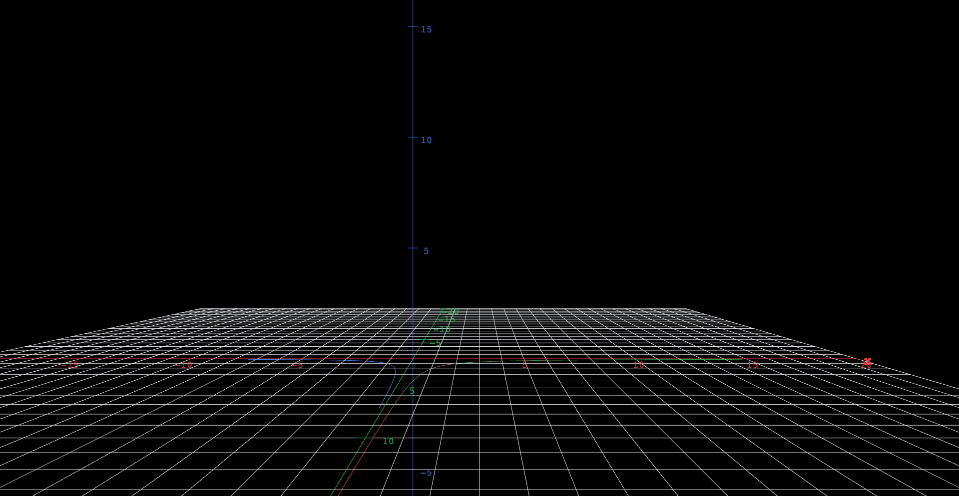
What does "both at once" look like? A solution is a moving point $(x(t), y(t))$ , and eliminating time exposes its path: the product $x(t)\,y(t) = x_0 y_0\, e^{t} e^{-t} = x_0 y_0$ never changes. Every orbit lies on a hyperbola $xy = c$ (or, when $c = 0$ , on an axis). The figure draws three of them.

Three hyperbola-shaped arcs in the plane, viewed face-on: a red and a green arc sweeping through the upper-right quadrant toward the horizontal axis, and a blue arc mirrored into the upper-left quadrant. Each arc rides in along the vertical axis direction and out along the horizontal axis direction, the signature flow of a saddle point at the origin. — Three orbits of the saddle system $x' = x$ , $y' = -y$ , viewed face-on, each drawn for $-2 \le t \le 2$ : red through $(1, 2)$ , green through $(2, 1)$ , and blue through $(-1, 1)$ . Each arc sweeps in along the vertical direction and out along the horizontal — the axes are the eigendirections, the only straight-line orbits.

Explore

Observe. Follow the red arc in the direction of increasing time. At $t = -2$ it sits at $(0.14, 14.8)$ , high against the vertical axis; by $t = 2$ it has swept down and out to $(7.4, 0.27)$ , flat along the horizontal. It falls in toward the origin, turns, and flees — and never actually arrives anywhere.
Predict. The red orbit passes through $(1, 2)$ and the green through $(2, 1)$ . Compute $xy$ for each point before looking closely: are these two different hyperbolas, or two pieces of the same one?
Verify. Both products equal $2$ — one hyperbola, $xy = 2$ . Check the shared point $(2, 1)$ : the red solution reaches it at $t = \ln 2 \approx 0.69$ , while the green solution starts there at $t = 0$ . Two different solutions, one orbit.
Observe. The blue arc, through $(-1, 1)$ , rides the branch $xy = -1$ in the second quadrant — the same shape, mirrored. Notice that no arc ever touches an axis: on the vertical axis $x = 0$ forces $x' = 0$ , so a state born on an axis stays on it forever. The eigendirections are invariant lines, and other orbits can only approach them.
Predict, then reason. Suppose both equations drained: $x' = -x$ , $y' = -y$ . No figure needed — what quantity is now constant along orbits in place of $xy$ , what shape are the orbits, and where does every state end up?

Connect

The example generalizes further than it looks. A general linear system $x' = ax + by$ , $y' = cx + dy$ hides its rates, but they are still there: along each eigendirection the motion is a pure exponential $e^{\lambda t}$ , and the pair of eigenvalues classifies the portrait completely. Real eigenvalues of opposite sign give a saddle — this figure: in along one direction, out along the other, hyperbolic arcs between. Real eigenvalues of the same sign give a node: every orbit sweeps into the origin (both negative) or out of it (both positive), with no way around. Complex eigenvalues $\alpha \pm i\beta$ give a spiral — rotation at rate $\beta$ with amplitude $e^{\alpha t}$ ; the phase loop of Chapter 2 was exactly this, eigenvalues $-a \pm ib$ . And purely imaginary eigenvalues give a center, the closed ellipses of the undamped spring. It is the damping-regime trichotomy again, wearing geometric clothes.

The portrait forgets the clock, and does so deliberately. Because the system is autonomous — time appears nowhere on the right-hand sides — delaying a solution produces another solution, and both trace the same curve. That is what the Explore steps uncovered: the green solution is the red one delayed by $\ln 2$ . An orbit is a road; a solution is a journey along it with a schedule. The phase portrait is the road map — every road, no schedules — and that economy is why one still image can hold every possible history of the system at once.

Example 1 A saddle in disguise

Classify the system $x' = y$ , $y' = x$ and find its orbits.

Nothing is decoupled here — but the combinations $u = x + y$ and $v = x - y$ are: $u' = x' + y' = y + x = u$ and $v' = x' - y' = y - x = -v$ . So $u = u_0 e^{t}$ and $v = v_0 e^{-t}$ : the same saddle as the figure, rotated onto new axes. The eigenvalues are again $1$ and $-1$ ; the eigendirections are the diagonals $y = x$ (growing) and $y = -x$ (decaying); and the conserved product is $uv = (x + y)(x - y) = x^2 - y^2$ , so the orbits are the hyperbolas $x^2 - y^2 = c$ . A state on the line $y = -x$ slides into the origin; a state anywhere else eventually escapes along the direction of $y = x$ . Keep this example in hand — it returns in the next section as the local picture beside a pendulum balanced upside down.

-1,\; 1

Eigenvalues of the saddle in disguise ✓ Computed · mojocas 0.1.0 ✓ Agrees with the text

The disguise removed by machine: the computer algebra system extracts both eigenvalues of the coupling matrix with certified multiplicities, confirming the rotated saddle the substitution $u = x + y$ , $v = x - y$ uncovered by hand.

Dial the Matrix

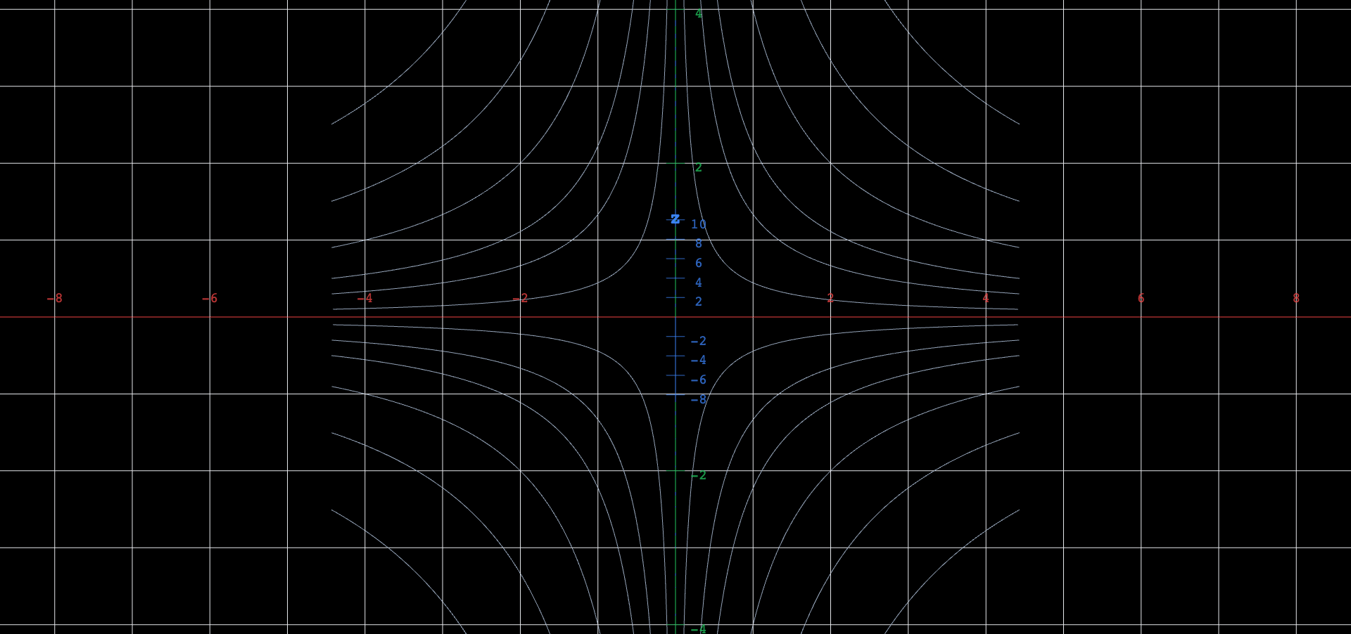
The classification above is a claim about every linear system, and three orbits of one system cannot show it. The figure below draws the whole portrait — a lattice of trajectories, computed rather than solved — for whatever matrix you dial in.

A square window centered on the origin, filled with solution trajectories launched from a lattice of starting points, each swept along whatever flow the four matrix entries currently dictate. At the starting settings the flow is the saddle of this section: trajectories fall in from top and bottom, turn as they near the origin, and flee left and right, so the family sketches a grid of hyperbolas and no trajectory ever reaches the centre. Dialing the four sliders re-draws every trajectory live — matching-sign settings pull all of them into the origin or push all of them out, and settings with rotation wind them into spirals or closed loops around it. — The phase portrait of $x' = ax + by$ , $y' = cx + dy$ , with all four matrix entries on sliders. It opens on $a = 1$ , $b = 0$ , $c = 0$ , $d = -1$ — this section's saddle. Every trajectory is integrated numerically, so the picture needs no solution formula.

Observe. At the opening settings, confirm the saddle: trajectories arrive along one axis, turn, and leave along the other. Which axis is the escaping direction, and does it match the eigenvalue $+1$ ?
Predict. Set $d = 1$ , so both diagonal entries are $+1$ . Before dragging, decide what every trajectory should do. Then drag, and name the portrait.
Verify. Now set $a = -1$ , $d = -1$ . Every orbit should sweep inward. This is a node; compare it with the saddle you started from and say precisely which sign change caused the difference.
Observe. Set $a = 0$ , $b = 1$ , $c = -1$ , $d = 0$ . The eigenvalues are $\pm i$ — purely imaginary. What shape appears, and why does "no real part" mean "neither growing nor decaying"?
Predict, then verify. From the centre in step 4, drag $a$ and $d$ together slightly negative. Purely imaginary eigenvalues acquire a small negative real part. Predict what the closed loops become, then check — and connect the result to the damped spring of Chapter 2.

I,\; -I

Purely imaginary eigenvalues of the centre ✓ Computed · mojocas 0.1.0 ✓ Agrees with the text

Step 4's matrix, handed to the computer algebra system: the eigenvalues come back exactly $\pm i$ — no real part to grow or decay, which is precisely why the portrait closes into loops.

An original work of XYZ Homework, built around interactive XYZ 3D figures, following the standard first-course sequence (first-order equations through systems and the phase plane). Distinct from the LibreTexts-sourced Differential Equations for Engineers (Lebl) edition, which has its own attribution. License: CC-BY-NC-SA-4.0.