0.2 Introduction to Differential Equations

Differential Equations

The laws of physics are generally written down as differential equations. Therefore, all of science and engineering use differential equations to some degree. Understanding differential equations is essential to understanding almost anything you will study in your science and engineering classes. You can think of mathematics as the language of science, and differential equations are one of the most important parts of this language as far as science and engineering are concerned. As an analogy, suppose all your classes from now on were given in Swahili. It would be important to first learn Swahili, or you would have a very tough time getting a good grade in your classes.

You saw many differential equations already without perhaps knowing about it. And you even solved simple differential equations when you took calculus. Let us see an example you may not have seen:

$\frac{d x}{d t} + x = 2 \cos t .$

(0.2.1)

Here

x

is the dependent variable and

t

is the independent variable. Equation (0.2.1) is a basic example of a differential equation. It is an example of a first order differential equation, since it involves only the first derivative of the dependent variable. This equation arises from Newton’s law of cooling where the ambient temperature oscillates with time.

Solutions of Differential Equations

Solving the differential equation means finding $x$ in terms of $t$ . That is, we want to find a function of $t$ , which we call $x$ , such that when we plug $x$ , $t$ , and $\frac{d x}{d t}$ into (0.2.1), the equation holds; that is, the left hand side equals the right hand side. It is the same idea as it would be for a normal (algebraic) equation of just $x$ and $t$ . We claim that

$x = x (t) = \cos t + \sin t$

is a solution. How do we check? We simply plug

x

into equation (0.2.1)! First we need to compute

\frac{d x}{d t}

. We find that

\frac{d x}{d t} = - \sin t + \cos t

. Now let us compute the left-hand side of (0.2.1).

$\frac{d x}{d t} + x = \underset{\frac{d x}{d t}}{\underset{⏟}{(- \sin t + \cos t)}} + \underset{x}{\underset{⏟}{(\cos t + \sin t)}} = 2 \cos t .$

Yay! We got precisely the right-hand side. But there is more! We claim

x = \cos t + \sin t + e^{- t}

is also a solution. Let us try,

$\frac{d x}{d t} = - \sin t + \cos t - e^{- t} .$

We plug into the left-hand side of (0.2.1)

$\frac{d x}{d t} + x = \underset{\frac{d x}{d t}}{\underset{⏟}{(- \sin t + \cos t - e^{- t})}} + \underset{x}{\underset{⏟}{(\cos t + \sin t + e^{- t})}} = 2 \cos t .$

And it works yet again!

So there can be many different solutions. For this equation all solutions can be written in the form

$x = \cos t + \sin t + C e^{- t},$

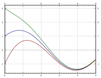
for some constant

C

. Different constants

C

will give different solutions, so there are really infinitely many possible solutions. See Figure

1

for the graph of a few of these solutions. We will see how we find these solutions a few lectures from now.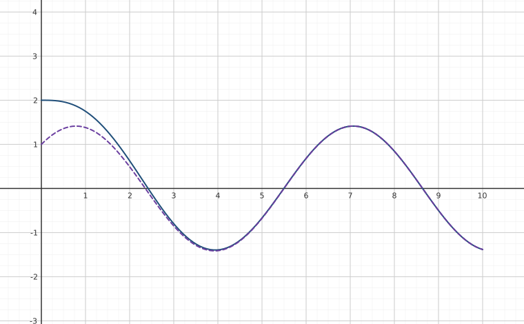

Function graph showing y = cos(t) + sin(t) + C*exp(-t) on t in [0, 10] and y = cos(t) + sin(t) on t in [0, 10]. Adjustable parameter: Constant C (C) = 1. Viewing window: x from -0.94 to 10.94, y from -3.07 to 4.27. — Every solution of equation (0.2.1): x = cos t + sin t + C·e^(-t), drawn against time t on the horizontal axis (XYZ Graph names the vertical axis y; here it is Lebl's x). Drag C from -3 to 3 and each curve leaves a different starting height at t = 0 - anywhere from -2 to 4, since x(0) = 1 + C - yet by t = 4 every one of them lies within 0.06 of the dashed C = 0 curve. The constant fixes only the transient; the long-run oscillation cos t + sin t is common to all of them. C = 1, the slider's starting value, is the solution the section checks by substitution.

Three solution curves over x from 0 to 5 starting at 3, 1 and -1. All fall through zero, bottom out near -1.45 around x = 3.95, then turn back up almost indistinguishably. — Figure $1$ : Few solutions of $\frac{d x}{d t} + x = 2 \cos t$ .

Solving differential equations can be quite hard. There is no general method that solves every differential equation. We will generally focus on how to get exact formulas for solutions of certain differential equations, but we will also spend a little bit of time on getting approximate solutions. And we will spend some time on understanding the equations without solving them.

Most of this book is dedicated to ordinary differential equations or ODEs, that is, equations with only one independent variable, where derivatives are only with respect to this one variable. If there are several independent variables, we get partial differential equations or PDEs.

Even for ODEs, which are very well understood, it is not a simple question of turning a crank to get answers. When you can find exact solutions, they are usually preferable to approximate solutions. It is important to understand how such solutions are found. Although in real applications you will leave much of the actual calculations to computers, you need to understand what they are doing. It is often necessary to simplify or transform your equations into something that a computer can understand and solve. You may even need to make certain assumptions and changes in your model to achieve this.

To be a successful engineer or scientist, you will be required to solve problems in your job that you never saw before. It is important to learn problem solving techniques, so that you may apply those techniques to new problems. A common mistake is to expect to learn some prescription for solving all the problems you will encounter in your later career. This course is no exception.

Differential Equations in Practice

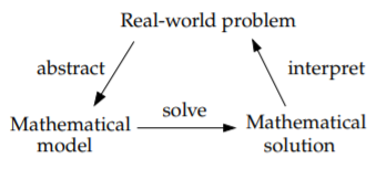
Diagram of a three-node cycle: an arrow labelled abstract runs from Real-world problem to Mathematical model, solve to Mathematical solution, and interpret back to the problem. — Figure $2$

So how do we use differential equations in science and engineering? First, we have some real-world problem we wish to understand. We make some simplifying assumptions and create a mathematical model. That is, we translate the real-world situation into a set of differential equations. Then we apply mathematics to get some sort of a mathematical solution. There is still something left to do. We have to interpret the results. We have to figure out what the mathematical solution says about the real-world problem we started with.

Learning how to formulate the mathematical model and how to interpret the results is what your physics and engineering classes do. In this course, we will focus mostly on the mathematical analysis. Sometimes we will work with simple real-world examples so that we have some intuition and motivation about what we are doing.

Let us look at an example of this process. One of the most basic differential equations is the standard exponential growth model. Let $P$ denote the population of some bacteria on a Petri dish. We assume that there is enough food and enough space. Then the rate of growth of bacteria is proportional to the population—a large population grows quicker. Let $t$ denote time (say in seconds) and $P$ the population. Our model is

$\frac{d P}{d t} = k P,$

for some positive constant

k greater than 0

Example 1

Suppose there are $100$ bacteria at time $0$ and $200$ bacteria $10$ seconds later. How many bacteria will there be $1$ minute from time $0$ (in $60$ seconds)?

Figure

2

: Bacteria growth in the first

60

seconds.

Show solution

First we need to solve the equation. We claim that a solution is given by

$P (t) = C e^{k t},$

where

C

is a constant. Let us try:

$\frac{d P}{d t} = C k e^{k t} = k P .$

And it really is a solution.

OK, now what? We do not know $C$ , and we do not know $k$ . But we know something. We know $P open parenthesis 0 close parenthesis equals 100$ , and we know $P open parenthesis 10 close parenthesis equals 200$ . Let us plug these conditions in and see what happens.

$\begin{matrix} 100 = P (0) = C e^{k 0} = C, \\ 200 = P (10) = 100 e^{k 10} . \end{matrix}$

Therefore,

2 = e^{10 k}

\frac{\ln 2}{10} = k \approx 0.069

. So

$P (t) = 100 e^{(\ln 2) t / 10} \approx 100 e^{0.069 t} .$

At one minute,

t equals 60

, the population is

P open parenthesis 60 close parenthesis equals 6400

. See Figure

2

Let us talk about the interpretation of the results. Does our solution mean that there must be exactly $6400$ bacteria on the plate at $60 s$ ? No! We made assumptions that might not be true exactly, just approximately. If our assumptions are reasonable, then there will be approximately $6400$ bacteria. Also, in real life $P$ is a discrete quantity, not a real number. However, our model has no problem saying that for example at $61$ seconds, $P open parenthesis 61 close parenthesis approximately equals 6859.35$ .

Normally, the $k$ in $P^{'} = k P$ is known, and we want to solve the equation for different initial conditions. What does that mean? Take $k equals 1$ for simplicity. Suppose we want to solve the equation $\frac{d P}{d t} = P$ subject to $P open parenthesis 0 close parenthesis equals 1000$ (the initial condition). Then the solution turns out to be (exercise)

$P (t) = 1000 e^{t} .$

We call $P (t) = C e^{t}$ the general solution, as every solution of the equation can be written in this form for some constant $C$ . We need an initial condition to find out what $C$ is, in order to find the particular solution we are looking for. Generally, when we say "particular solution," we just mean some solution.

Fundamental Equations

A few equations appear often and it is useful to just memorize what their solutions are. Let us call them the four fundamental equations. Their solutions are reasonably easy to guess by recalling properties of exponentials, sines, and cosines. They are also simple to check, which is something that you should always do. No need to wonder if you remembered the solution correctly.

Function graph showing y = exp(k*x), y = exp(-k*x), y = cos(k*x) and y = cosh(k*x). Adjustable parameter: Rate / frequency k (k) = 1. Viewing window: x from -5.28 to 5.28, y from -2.26 to 4.26. — The section's four fundamental equations on one set of axes, all driven by a single shared k. The curve rising to the right is e^(kx), solving y′ = ky; its mirror image rising to the left is e^(-kx), solving y′ = -ky; the wave is cos(kx), solving y″ = -k²y; and the dashed curve is cosh(kx) = (e^(kx) + e^(-kx))/2, solving y″ = k²y — which is why it runs exactly halfway between the two exponentials at every x. All four pass through y = 1 at x = 0, whatever k is. Lebl takes k > 0; drag the slider down to the degenerate k = 0 and the four equations become the same equation, so all four curves collapse onto the single line y = 1. Drag k up to 2 and the wave stays trapped between -1 and 1 while the other three leave the top of the frame ever sooner — but they were already unbounded back at k = 0.1, so what separates oscillation from blow-up is the minus sign on k² in y″ = -k²y, not the size of k. The minus in y′ = -ky buys nothing: it only flips which side e^(-kx) blows up on.

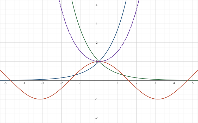
First such equation is

$\frac{d y}{d x} = k y,$

for some constant

k greater than 0

. Here

y

is the dependent and

x

the independent variable. The general solution for this equation is

$y (x) = C e^{k x} .$

We saw above that this function is a solution, although we used different variable names.

Next,

$\frac{d y}{d x} = - k y,$

for some constant

k greater than 0

. The general solution for this equation is

$y (x) = C e^{- k x} .$

Next, take the second order differential equation

$\frac{d^{2} y}{{d x}^{2}} = - k^{2} y,$

for some constant

k greater than 0

. The general solution for this equation is

$y (x) = C_{1} \cos (k x) + C_{2} \sin (k x) .$

Since the equation is a second order differential equation, we have two constants in our general solution.

Finally, consider the second order differential equation

$\frac{d^{2} y}{{d x}^{2}} = k^{2} y,$

for some constant

k greater than 0

. The general solution for this equation is

$y (x) = C_{1} e^{k x} + C_{2} e^{- k x},$

$y (x) = D_{1} \cosh (k x) + D_{2} \sinh (k x) .$

For those that do not know, $\cosh$ and $\sinh$ are defined by

$\cosh x = \frac{e^{x} + e^{- x}}{2}, \sinh x = \frac{e^{x} - e^{- x}}{2} .$

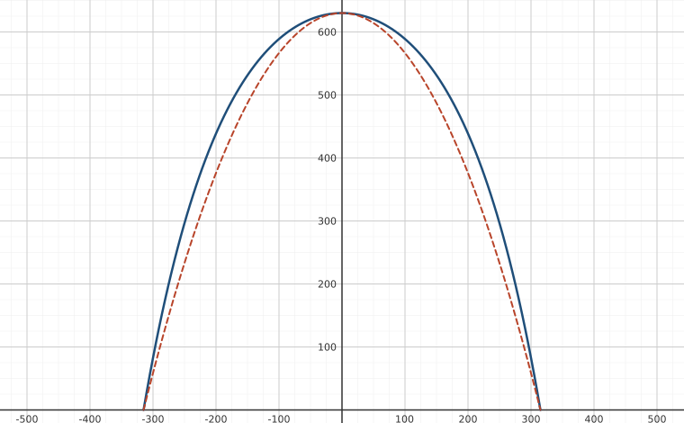
They are called the hyperbolic cosine and hyperbolic sine. These functions are sometimes easier to work with than exponentials. They have some nice familiar properties such as

cosh 0 equals 1

sinh 0 equals 0

, and

\frac{d}{d x} \cosh x = \sinh x

(no that is not a typo) and

\frac{d}{d x} \sinh x = \cosh x

An interesting note about $\cosh$ : The graph of $\cosh$ is the exact shape of a hanging chain. This shape is called a catenary. Contrary to popular belief this is not a parabola. If you invert the graph of $\cosh$ , it is also the ideal arch for supporting its weight. For example, the gateway arch in Saint Louis is an inverted graph of $\cosh$ —if it were just a parabola it might fall. The formula used in the design is inscribed inside the arch:

$y = - 127.7 ft \cdot \cosh (x / 127.7 ft) + 757.7 ft .$

Function graph showing y = 630*(cosh(315/a) - cosh(x/a))/(cosh(315/a) - 1) on x in [-315, 315] and y = 630*(1 - (x/315)^2) on x in [-315, 315]. Adjustable parameter: Catenary scale a (a) = 127.7 ft. Viewing window: x from -542.86 to 542.86, y from -20.71 to 650.71. — The arch this section prints, y = 630(cosh(315/a) − cosh(x/a))/(cosh(315/a) − 1), against the parabola through the same two feet (x = ±315 ft) and the same 630 ft apex — so the slider changes nothing but the shape. Lebl's own constants put the arch 630 ft tall over a 630 ft span, and at a = 127.7 ft the catenary rides about 66 ft above the parabola near x = 228 ft, a tenth of the arch's height. Drag a down to 60 and the gap opens past 190 ft; drag it up to 600 and it closes to under 4 ft, since cosh u ≈ 1 + u²/2 once u is small. That last picture is why the popular belief survives — a flat enough catenary is a parabola to the eye. This one is not flat.

Adapted from Differential Equations for Engineers by Jiří Lebl (Oklahoma State University), hosted on LibreTexts (math.libretexts.org) and licensed under CC BY-SA 4.0. Changes were made. License: CC-BY-SA-4.0.