8.1 More Probability

Chapter Overview

In this chapter, you will learn to:

Find the probability of a binomial experiment.
Find probabilities using Bayes' Formula.
Find the expected value or payoff in a game of chance.
Find probabilities using tree diagrams.

Binomial Probability

In this section, we will consider types of problems that involve a sequence of trials, where each trial has only two outcomes, a success or a failure. These trials are independent, that is, the outcome of one does not affect the outcome of any other trial. Furthermore, the probability of success, $p$ , and the probability of failure, $open parenthesis 1 minus p close parenthesis$ , remains the same throughout the experiment. These problems are called binomial probability problems. Since these problems were researched by a Swiss mathematician named Jacques Bernoulli around 1700, they are also referred to as Bernoulli trials.

We give the following definition:

Binomial Experiment A binomial experiment satisfies the following four conditions:

There are only two outcomes, a success or a failure, for each trial.
The same experiment is repeated several times.
The trials are independent; that is, the outcome of a particular trial does not affect the outcome of any other trial.
The probability of success remains the same for every trial.

The probability model that we are about to investigate will give us the tools to solve many real-life problems like the ones given below.

If a coin is flipped 10 times, what is the probability that it will fall heads 3 times?
If a basketball player makes 3 out of every 4 free throws, what is the probability that he will make 7 out of 10 free throws in a game?
If a medicine cures 80% of the people who take it, what is the probability that among the ten people who take the medicine, 6 will be cured?
If a microchip manufacturer claims that only 4% of his chips are defective, what is the probability that among the 60 chips chosen, exactly three are defective?
If a telemarketing executive has determined that 15% of the people contacted will purchase the product, what is the probability that among the 12 people who are contacted, 2 will buy the product?

We now consider the following example to develop a formula for finding the probability of $k$ successes in n Bernoulli trials.

Example 1

A baseball player has a batting average of $.300$ . If he bats four times in a game, find the probability that he will have

four hits
three hits
two hits
one hit
no hits.

Let us suppose $S$ denotes that the player gets a hit, and $F$ denotes that he does not get a hit.

This is a binomial experiment because it meets all four conditions. First, there are only two outcomes, $S$ or $F$ . Clearly the experiment is repeated four times. Lastly, if we assume that the player's skillfulness to get a hit does not change each time he comes to bat, the trials are independent with a probability of $.3$ of getting a hit during each trial.

We draw a tree diagram to show all situations.

Figure 8.1

Let us first find the probability of getting, for example, two hits. We will have to consider the six possibilities, $SSFF$ , $SFSF$ , $SFFS$ , $FSSF$ , $FSFS$ , $FFSS$ , as shown in the above tree diagram. We list the probabilities of each below.

$P (SSFF) = (. 3) (. 3) (. 7) (. 7) = {(. 3)}^{2} {(. 7)}^{2}$

$P (SFSF) = (. 3) (. 7) (. 3) (. 7) = {(. 3)}^{2} {(. 7)}^{2}$

$P (SFFS) = (. 3) (. 7) (. 7) (. 3) = {(. 3)}^{2} {(. 7)}^{2}$

$P (FSSF) = (. 7) (. 3) (. 3) (. 7) = {(. 3)}^{2} {(. 7)}^{2}$

$P (FSFS) = (. 7) (. 3) (. 7) (. 3) = {(. 3)}^{2} {(. 7)}^{2}$

$P (FFSS) = (. 7) (. 7) (. 3) (. 3) = {(. 3)}^{2} {(. 7)}^{2}$

Since the probability of each of these six outcomes is $open parenthesis .3 close parenthesis squared open parenthesis .7 close parenthesis squared$ , the probability of obtaining two successes is $6 open parenthesis .3 close parenthesis squared open parenthesis .7 close parenthesis squared$ .

The probability of getting one hit can be obtained in the same way. Since each permutation has one $S$ and three $F$ 's, there are four such outcomes: $SFFF$ , $FSFF$ , $FFSF$ , and $FFFS$ .

And since the probability of each of the four outcomes is $open parenthesis .3 close parenthesis open parenthesis .7 close parenthesis cubed$ , the probability of getting one hit is $4 open parenthesis .3 close parenthesis open parenthesis .7 close parenthesis cubed$ .

The table below lists the probabilities for all cases, and shows a comparison with the binomial expansion of fourth degree. Again, $p$ denotes the probability of success, and $q = (1 - p)$ the probability of failure.

**Table 8.1**
Outcome	Four Hits	Three hits	Two Hits	One hits	No Hits
Probability	$open parenthesis .3 close parenthesis to the power 4$	$4 open parenthesis .3 close parenthesis cubed open parenthesis .7 close parenthesis$	$6 open parenthesis .3 close parenthesis squared open parenthesis .7 close parenthesis squared$	$4 open parenthesis .3 close parenthesis open parenthesis .7 close parenthesis cubed$	$open parenthesis .7 close parenthesis to the power 4$

This gives us the following theorem:

We use the above formula to solve the following examples.

Bayes' Formula

In this section, we will develop and use Bayes' Formula to solve an important type of probability problem. Bayes' formula is a method of calculating the conditional probability $P open parenthesis F ∣ E close parenthesis$ from $P open parenthesis E ∣ F close parenthesis$ . The ideas involved here are not new, and most of these problems can be solved using a tree diagram. However, Bayes' formula does provide us with a tool with which we can solve these problems without a tree diagram.

We begin with an example.

Example 7

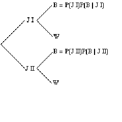
Suppose you are given two jars. Jar I contains one black and 4 white marbles, and Jar II contains 4 black and 6 white marbles. If a jar is selected at random and a marble is chosen,

What is the probability that the marble chosen is a black marble?
If the chosen marble is black, what is the probability that it came from Jar I?
If the chosen marble is black, what is the probability that it came from Jar II?

Let $J I$ I be the event that Jar I is chosen, $J II$ be the event that Jar II is chosen, $B$ be the event that a black marble is chosen and $W$ the event that a white marble is chosen.

We illustrate using a tree diagram.

Figure 8.2

The probability that a black marble is chosen is $P (B) = 1 / 10 + 2 / 10 = 3 / 10$ .
To find $P open parenthesis J I ∣ B close parenthesis$ , we use the definition of conditional probability, and we get
$P (J I ∣ B) = \frac{P (J I \cap B)}{P (B)} = \frac{1 / 10}{3 / 10} = \frac{1}{3}$
Similarly, $P (J II ∣ B) = \frac{P (J II \cap B)}{P (B)} = \frac{2 / 10}{3 / 10} = \frac{2}{3}$
In parts b and c, the reader should note that the denominator is the sum of all probabilities of all branches of the tree that produce a black marble, while the numerator is the branch that is associated with the particular jar in question.

We will soon discover that this is a statement of Bayes' formula.

Let us first visualize the problem.

We are given a sample space $S$ and two mutually exclusive events $J I$ and $J II$ . That is, the two events, $J I$ and $J II$ , divide the sample space into two parts such that $J I \cup J II = S$ . Furthermore, we are given an event $B$ that has elements in both $J I$ and $J II$ , as shown in the tree diagram below.

Tree diagram with two first-stage branches, Jar I and Jar II. Each jar branches to a black marble B or a white marble W. The black-marble outcomes are labeled B = P(J I)P(B | J I) for Jar I and B = P(J II)P(B | J II) for Jar II. — **Figure 8.3**

From the Venn diagram, we can see that

$B = (B \cap J I) \cup (B \cap J II)$

and

$P (B) = P (B \cap J I) + P (B \cap J II)$

But the product rule in the related section gives us

$P (B \cap J I) = P (J I) \cdot P (B ∣ J I)$ $P (B \cap J II) = P (J II) \cdot P (B ∣ J II)$

Substituting in, we get

$P (B) = P (J I) \cdot P (B ∣ J I) + P (J II) \cdot P (B ∣ J II)$

The conditional probability formula gives us

$P (J I ∣ B) = \frac{P (J I \cap B)}{P (B)}$

Therefore,

$P (J I ∣ B) = \frac{P (J I \cdot P (B ∣ J I))}{P (B)}$

or,

$P (J I ∣ B) = \frac{P (J I) \cdot P (B ∣ J I)}{P (J I) \cdot P (B ∣ J I) + P (J II) \cdot P (B ∣ J II)}$

The last statement is Bayes' Formula for the case where the sample space is divided into two partitions. The following is the generalization of this formula for n partitions.

Example 8

Let $S$ be a sample space that is divided into $n$ partitions, $A sub 1$ , $A sub 2$ ,... $A_{n}$ . If $E$ is any event in $S$ , then

$P (A_{i} ∣ E) = \frac{P (A_{i}) P (E ∣ A_{i})}{P (A_{1}) P (E ∣ A_{1}) + P (A_{2}) P (E ∣ A_{2}) + \dots + P (A_{n}) P (E ∣ A_{n})}$

We begin with the following example.

Example 9

A department store buys 50% of its appliances from Manufacturer A, 30% from Manufacturer B, and 20% from Manufacturer C. It is estimated that 6% of Manufacturer A's appliances, 5% of Manufacturer B's appliances, and 4% of Manufacturer C's appliances need repair before the warranty expires. An appliance is chosen at random. If the appliance chosen needed repair before the warranty expired, what is the probability that the appliance was manufactured by Manufacturer A? Manufacturer B? Manufacturer C?

Let events $A$ , $B$ and $C$ be the events that the appliance is manufactured by Manufacturer A, Manufacturer B, and Manufacturer C, respectively. Further, suppose that the event $R$ denotes that the appliance needs repair before the warranty expires.

We need to find $P open parenthesis A ∣ R close parenthesis$ , $P open parenthesis B ∣ R close parenthesis$ and $P open parenthesis C ∣ R close parenthesis$ .

We will do this problem both by using a tree diagram and by using Bayes' formula.

We draw a tree diagram.

Figure 8.4

The probability $P open parenthesis A ∣ R close parenthesis$ , for example, is a fraction whose denominator is the sum of all probabilities of all branches of the tree that result in an appliance that needs repair before the warranty expires, and the numerator is the branch that is associated with Manufacturer A. $P open parenthesis B ∣ R close parenthesis$ and $P open parenthesis C ∣ R close parenthesis$ are found in the same way. We list both as follows:

$P (A ∣ R) = \frac{. 030}{(. 030) + (. 015) + (. 008)} = \frac{. 030}{. 053} = . 566$

$P (B ∣ R) = \frac{. 015}{. 053} = . 283$ and $P (C ∣ R) = \frac{. 008}{. 053} = . 151$ .

Alternatively, using Bayes' formula,

$\begin{matrix} P (A ∣ R) = \frac{P (A) P (R ∣ A)}{P (A) P (R ∣ A) + P (B) P (R ∣ B) + P (C) P (R ∣ C)} \\ = \frac{. 030}{(. 030) + (. 015) + (. 008)} = \frac{. 030}{. 053} = . 566 \end{matrix}$

$P open parenthesis B ∣ R close parenthesis$ and $P open parenthesis C ∣ R close parenthesis$ can be determined in the same manner.

Example 10

There are five Jacy's department stores in San Jose. The distribution of number of employees by gender is given in the table below.

**Table 8.2**
Store Number	Number of Employees	Percent of Women Employees
1	300	.40
2	150	.65
3	200	.60
4	250	.50
5	100	.70
	Total=1000

If an employee chosen at random is a woman, what is the probability that the employee works at store III?

Let $k equals 1,2,..., 5$ be the event that the employee worked at store $k$ , and $W$ be the event that the employee is a woman. Since there are a total of 1000 employees at the five stores,

$P (1) = . 30 P (2) = . 15 P (3) = . 20 P (4) = . 25 P (5) = . 10$

Using Bayes' formula,

$\begin{array}{l} P (3, ∣, W) & = & \frac{P (3) P (W, ∣, 3)}{P (1) P (W, ∣, 1) + P (2) P (W, ∣, 2) + P (3) P (W, ∣, 3) + P (4) P (W, ∣, 4) + P (5) P (W, ∣, 5)} \\ = & \frac{(., 20) (., 60)}{(., 30) (., 40) + (., 15) (., 65) + (., 20) (., 60) + (., 25) (., 50) + (., 10) (., 70)} \\ = & . 2254 \end{array}$

Expected Value

An expected gain or loss in a game of chance is called Expected Value. The concept of expected value is closely related to a weighted average. Consider the following situations.

Suppose you and your friend play a game that consists of rolling a die. Your friend offers you the following deal: If the die shows any number from 1 to 5, he will pay you the face value of the die in dollars, that is, if the die shows a 4, he will pay you $4. But if the die shows a 6, you will have to pay him $18.
Before you play the game you decide to find the expected value. You analyze as follows.
Since a die will show a number from 1 to 6, with an equal probability of $1 / 6$ , your chance of winning $1 is $1 / 6$ , winning $2 is $1 / 6$ , and so on up to the face value of 5. But if the die shows a 6, you will lose $18. You write the expected value.
$E = $ 1 (1 / 6) + $ 2 (1 / 6) + $ 3 (1 / 6) + $ 4 (1 / 6) + $ 5 (1 / 6) - $ 18 (1 / 6) = - $ . 50$
This means that every time you play this game, you can expect to lose 50 cents. In other words, if you play this game 100 times, theoretically you will lose $50. Obviously, it is not to your interest to play.
Suppose of the ten quizzes you took in a course, on eight quizzes you scored 80, and on two you scored 90. You wish to find the average of the ten quizzes. The average is
$A = \frac{(80) (8) + (90) (2)}{10} = (80) \frac{8}{10} + (90) \frac{2}{10} = 82$
It should be observed that it will be incorrect to take the average of 80 and 90 because you scored 80 on eight quizzes, and 90 on only two of them. Therefore, you take a "weighted average" of 80 and 90. That is, the average of 8 parts of 80 and 2 parts of 90, which is 82.

In the first situation, to find the expected value, we multiplied each payoff by the probability of its occurrence, and then added up the amounts calculated for all possible cases. In the second part of, if we consider our test score a payoff, we did the same. This leads us to the following definition.

Example 11

In a town, 10% of the families have three children, 60% of the families have two children, 20% of the families have one child, and 10% of the families have no children. What is the expected number of children to a family?

We list the information in the following table.

**Table 8.3**
Number of Children	3	2	1	0
Probability	$.10$	$.60$	$.20$	$.10$

$Expected Value = x_{1} p (x_{1}) + x_{2} p (x_{2}) + x_{3} p (x_{3}) + x_{4} p (x_{4})$

$E = 3 (. 10) + 2 (. 60) + 1 (. 20) + 0 (. 10) = 1 . 7$

So on average, there are 1.7 children to a family.

Example 12

To sell an average house, a real estate broker spends $1200 for advertisement expenses. If the house sells in three months, the broker makes $8,000. Otherwise, the broker loses the listing. If there is a 40% chance that the house will sell in three months, what is the expected payoff for the real estate broker?

The broker makes $8,000 with a probability of $.40$ , but he loses $1200 whether the house sells or not.

$E = ($ . 8000) (. 40) - ($ 1200) = $ 2, 000$ .

Alternatively, the broker makes $$ open parenthesis 8000 minus 1200 close parenthesis$ with a probability of $.40$ , but loses $1200 with a probability of $.60$ . Therefore,

$E = ($ 6800) (. 40) - ($ 1200) (. 60) = $ 2, 000$ .

Probability Using Tree Diagrams

As we have already seen, tree diagrams play an important role in solving probability problems. A tree diagram helps us not only visualize, but also list all possible outcomes in a systematic fashion. Furthermore, when we list various outcomes of an experiment and their corresponding probabilities on a tree diagram, we gain a better understanding of when probabilities are multiplied and when they are added. The meanings of the words and and or become clear when we learn to multiply probabilities horizontally across branches, and add probabilities vertically down the tree.

Although tree diagrams are not practical in situations where the possible outcomes become large, they are a significant tool in breaking the problem down in a schematic way. We consider some examples that may seem difficult at first, but with the help of a tree diagram, they can easily be solved.

Example 15

A person has four keys and only one key fits to the lock of a door. What is the probability that the locked door can be unlocked in at most three tries?

Let $U$ be the event that the door has been unlocked and $L$ be the event that the door has not been unlocked. We illustrate with a tree diagram.

Figure 8.5

$The probability of unlocking the door in the first try = 1/4$

$The probability of unlocking the door in the second try = (3 / 4) (1 / 3) = 1 / 4$

$The probability of unlocking the door in the third try = (3 / 4) (2 / 3) (1 / 2) = 1 / 4$

Therefore, $the probability of unlocking the door in at most three tries = 1 / 4 + 1 / 4 + 1 / 4 = 3 / 4$

Example 17

A circuit consists of three resistors: resistor $R sub 1$ , resistor $R sub 2$ , and resistor $R sub 3$ , joined in a series. If one of the resistors fails, the circuit stops working. If the probability that resistors $R sub 1$ , $R sub 2$ , or $R sub 3$ will fail is $.07$ , $.10$ , and $.08$ , respectively, what is the probability that at least one of the resistors will fail?

Clearly, $the that at least one of the resistors fails = 1 - none of the resistors fails$ .

It is quite easy to find the probability of the event that none of the resistors fails. We don't even need to draw a tree because we can visualize the only branch of the tree that assures this outcome.

The probabilities that $R sub 1$ , $R sub 2$ , $R sub 3$ will not fail are $.93$ , $.90$ , and $.92$ respectively. Therefore, $the probability that none of the resistors fails = (. 93) (. 90) (. 92) = . 77$ .

Thus, $the probability that at least one of them will fail = 1 - . 77 = . 23$ .

Adapted from Applied Finite Mathematics by Rupinder Sekhon (De Anza College), originally published by OpenStax CNX (cnx.org, collection col10613), licensed under CC BY 3.0. Changes were made. License: CC-BY-3.0.