3.1 Linear Programming: A Geometric Approach

Chapter Overview

In this chapter, you will learn to:

1. Solve linear programming problems that maximize the objective function.
2. Solve linear programming problems that minimize the objective function.

Maximization Applications

Application problems in business, economics, and social and life sciences often ask us to make decisions on the basis of certain conditions. These conditions or constraints often take the form of inequalities. In this section, we will look at such problems.

A typical linear programming problem consists of finding an extreme value of a linear function subject to certain constraints. We are either trying to maximize or minimize our function. That is why these linear programming problems are classified as maximization or minimization problems, or just optimization problems. The function we are trying to optimize is called an objective function, and the conditions that must be satisfied are called constraints. In this chapter, we will do problems that involve only two variables, and therefore, can be solved by graphing. We begin by solving a maximization problem.

Although we are mostly focusing on the standard maximization problems where all constraints are of the form , we will now consider an example where that is not the case.

Finally, we address an important question. Is it possible to determine the point that gives the maximum value without calculating the value at each critical point?

The answer is yes.

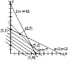
For example, in the above problem, we substituted the points (0, 0), (0, 6), (2, 5), (5, 2), and (6, 0), in the objective function $P=\text{20}x+\text{30}y$, and we got the values $0, $180, $190, $160, $120, respectively. Sometimes that is not the most efficient way of finding the optimum solution.

To determine the largest $P$, we graph $P=\text{20}x+\text{30}y$ for any value $P$ of our choice. Let us say, we choose $P=\text{60}$. We graph $\text{20}x+\text{30}y=\text{60}$. Now we move the line parallel to itself, that is, keeping the same slope at all times. Since we are moving the line parallel to itself, the slope is kept the same, and the only thing that is changing is the $P$. As we move away from the origin, the value of $P$ increases. The largest value of $P$ is realized when the line touches the last corner point. The figure below shows the movements of the line, and the optimum solution is achieved at the point (2, 5). In maximization problems, as the line is being moved away from the origin, this optimum point is the farthest critical point.

We summarize:

Minimization Applications

Minimization linear programming problems are solved in much the same way as the maximization problems. For the standard minimization linear programming problem, the constraints are of the form $\text{ax}+\text{by}\ge c$, as opposed to the form for the standard maximization problem. As a result, the feasible solution extends indefinitely to the upper right of the first quadrant, and is unbounded. But that is not a concern, since in order to minimize the objective function, the line associated with the objective function is moved towards the origin, and the critical point that minimizes the function is closest to the origin.

However, one should be aware that in the case of an unbounded feasibility region, the possibility of no optimal solution exists.

Although the method of solving minimization problems is similar to that of the maximization problems, we still feel that we should summarize the steps involved.