2.1 Matrices

Chapter Overview

In this chapter, you will learn to:

Do matrix operations.
Solve linear systems using the Gauss-Jordan method.
Solve linear systems using the matrix inverse method.
Do application problems.

Introduction to Matrices

Section Overview

In this section you will learn to:

Add and subtract matrices.
Multiply a matrix by a scalar.
Multiply two matrices.

A matrix is a rectangular array of numbers. Matrices are useful in organizing and manipulating large amounts of data. In order to get some idea of what matrices are all about, we will look at the following example.

Example 1

Fine Furniture Company makes chairs and tables at its San Jose, Hayward, and Oakland factories. The total production, in hundreds, from the three factories for the years 2024 and 2025 is listed in the table below.

Table 2.1

San Jose

Hayward

Oakland

Represent the production for the years 2024 and 2025 as the matrices A and B.
Find the difference in sales between the years 2024 and 2025.
The company predicts that in the year 2030 the production at these factories will double that of the year 2024. What will the production be for the year 2030?

The matrices are as follows: $A equals open bracket 30, 18; 20, 12; 16, 10 close bracket$ $B equals open bracket 36, 20; 24, 18; 20, 12 close bracket$
We are looking for the matrix $B - A$ . When two matrices have the same number of rows and columns, the matrices can be added or subtracted entry by entry. Therefore, we get
$B - A = [\begin{matrix} 36 - 30 & 20 - 18 \\ 24 - 20 & 18 - 12 \\ 20 - 16 & 12 - 10 \end{matrix}] = [\begin{matrix} 6 & 2 \\ 4 & 6 \\ 4 & 2 \end{matrix}]$
We would like a matrix that is twice the matrix of 2024, i.e., $2A$ .
Whenever a matrix is multiplied by a number, each entry is multiplied by the number.
$2A = 2 [\begin{matrix} 30 & 18 \\ 20 & 12 \\ 16 & 10 \end{matrix}] = [\begin{matrix} 60 & 36 \\ 40 & 24 \\ 32 & 20 \end{matrix}]$

Before we go any further, we need to familiarize ourselves with some terms that are associated with matrices. The numbers in a matrix are called the entries or the elements of a matrix. Whenever we talk about a matrix, we need to know the size or the dimension of the matrix. The dimension of a matrix is the number of rows and columns it has. When we say a matrix is a 3 by 4 matrix, we are saying that it has 3 rows and 4 columns. The rows are always mentioned first and the columns second. This means that a $3 times 4$ matrix does not have the same dimension as a $4 times 3$ matrix. A matrix that has the same number of rows as columns is called a square matrix. A matrix with all entries zero is called a zero matrix. A square matrix with 1's along the main diagonal and zeros everywhere else, is called an identity matrix. When a square matrix is multiplied by an identity matrix of same size, the matrix remains the same. A matrix with only one row is called a row matrix or a row vector, and a matrix with only one column is called a column matrix or a column vector. Two matrices are equal if they have the same size and the corresponding entries are equal.

Matrix Addition and Subtraction

If two matrices have the same size, they can be added or subtracted. The operations are performed on corresponding entries.

Example 2

Given the matrices $A$ , $B$ , $C$ and $D$ , below

$A = [\begin{matrix} 1 & 2 & 4 \\ 2 & 3 & 1 \\ 5 & 0 & 3 \end{matrix}] B = [\begin{matrix} 2 & - 1 & 3 \\ 2 & 4 & 2 \\ 3 & 6 & 1 \end{matrix}] C = [\begin{matrix} 4 \\ 2 \\ 3 \end{matrix}] D = [\begin{matrix} - 2 \\ - 3 \\ 4 \end{matrix}]$

Find, if possible.

$A + B$
$C - D$
$A + D$ .

As we mentioned earlier, matrix addition and subtraction involves performing these operations entry by entry.

We add each element of $A$ to the corresponding entry of $B$ .
$A + B = [\begin{matrix} 3 & 1 & 7 \\ 4 & 7 & 3 \\ 8 & 6 & 4 \end{matrix}]$
Just like the problem above, we perform the subtraction entry by entry.
$C - D = [\begin{matrix} 6 \\ 5 \\ - 1 \end{matrix}]$
The sum $A + D$ cannot be found because the two matrices have different sizes.

Multiplying a Matrix by a Scalar

If a matrix is multiplied by a scalar (a constant number), each entry is multiplied by that scalar.

Multiplication of Two Matrices

To multiply a matrix by another is not as easy as the addition, subtraction, or scalar multiplication of matrices. Because of its wide use in application problems, it is important that we learn it well. Therefore, we will try to learn the process in a step by step manner. We first begin by finding a product of a row matrix and a column matrix.

Example 6

Given $A equals open bracket 2, 3, 4 close bracket$ and $B equals open bracket 5, 3; 6, 4; 7, 5 close bracket$ , find the product $AB$ .

We already know how to multiply a row matrix by a column matrix. To find the product $AB$ , in this example, we will be multiplying the row matrix $A$ to both the first and second columns of matrix $B$ , resulting in a $1 times 2$ matrix.

$AB = [\begin{matrix} 2 \cdot 5 + 3 \cdot 6 + 4 \cdot 7 & 2 \cdot 3 + 3 \cdot 4 + 4 \cdot 5 \end{matrix}] = [\begin{matrix} 56 & 38 \end{matrix}]$

We have just multiplied a $1 times 3$ matrix by a matrix whose size is $3 times 2$ . So unlike addition and subtraction, it is possible to multiply two matrices with different dimensions as long as the number of entries in the rows of the first matrix are the same as the number of entries in columns of the second matrix.

Example 7

Given $A equals open bracket 2, 3, 4; 1, 2, 3 close bracket$ and $B equals open bracket 5, 3; 6, 4; 7, 5 close bracket$ , find the product $AB$ .

This time we are multiplying two rows of the matrix $A$ with two columns of the matrix $B$ . Since the number of entries in each row of $A$ are the same as the number of entries in each column of $B$ , the product is possible. We do exactly what we did in Example 6. The only difference is that the matrix $A$ has one more row.

We multiply the first row of the matrix $A$ with the two columns of $B$ , one at a time, and then repeat the process with the second row of $A$ . We get

$\begin{matrix} AB & = & [\begin{matrix} 2 & 3 & 4 \\ 1 & 2 & 3 \end{matrix}] [\begin{matrix} 5 & 3 \\ 6 & 4 \\ 7 & 5 \end{matrix}] \\ = & [\begin{matrix} 2 \cdot 5 + 3 \cdot 6 + 4 \cdot 7 & 2 \cdot 3 + 3 \cdot 4 + 4 \cdot 5 \\ 1 \cdot 5 + 2 \cdot 6 + 3 \cdot 7 & 1 \cdot 3 + 2 \cdot 4 + 3 \cdot 5 \end{matrix}] \\ = & [\begin{matrix} 56 & 38 \\ 38 & 26 \end{matrix}] \end{matrix}$

Example 8

Given the matrices $E$ , $F$ , $G$ and $H$ , below

$E = [\begin{matrix} 1 & 2 \\ 4 & 2 \\ 3 & 1 \end{matrix}] F = [\begin{matrix} 2 & - 1 \\ 3 & 2 \end{matrix}] G = [\begin{matrix} 4 & 1 \end{matrix}] H = [\begin{matrix} - 3 \\ - 1 \end{matrix}]$

Find, if possible.

$EF$
$FE$
$FH$
$GH$

To find $EF$ , we multiply the first row $open bracket 1, 2 close bracket$ of $E$ with the columns $open bracket 2; 3 close bracket$ and $open bracket minus 1; 2 close bracket$ of the matrix $F$ , and then repeat the process by multiplying the other two rows of $E$ with these columns of $F$ . The result is as follows:
$\begin{matrix} EF & = & [\begin{matrix} 1 & 2 \\ 4 & 2 \\ 3 & 1 \end{matrix}] [\begin{matrix} 2 & - 1 \\ 3 & 2 \end{matrix}] \\ = & [\begin{matrix} 1 \cdot 2 + 2 \cdot 3 & 1 \cdot - 1 + 2 \cdot 2 \\ 4 \cdot 2 + 2 \cdot 3 & 4 \cdot - 1 + 2 \cdot 2 \\ 3 \cdot 2 + 1 \cdot 3 & 3 \cdot - 1 + 1 \cdot 2 \end{matrix}] = [\begin{matrix} 8 & 3 \\ 14 & 0 \\ 9 & - 1 \end{matrix}] \end{matrix}$
The product $FE$ is not possible because the matrix $F$ has two entries in each row, while the matrix $E$ has three entries in each column. In other words, the matrix $F$ has two columns, while the matrix $E$ has three rows.
$FH = [\begin{matrix} 2 & - 1 \\ 3 & 2 \end{matrix}] [\begin{matrix} - 3 \\ - 1 \end{matrix}] = [\begin{matrix} 2 \cdot - 3 + - 1 \cdot - 1 \\ 3 \cdot - 3 + 2 \cdot - 1 \end{matrix}] = [\begin{matrix} - 5 \\ - 11 \end{matrix}]$
$GH = [\begin{matrix} 4 & 1 \end{matrix}] [\begin{matrix} - 3 \\ - 1 \end{matrix}] = [4 \cdot - 3 + 1 \cdot - 1] = [- 13]$

We summarize matrix multiplication as follows:

In order for product $AB$ to exist, the number of columns of $A$ , must equal the number of rows of $B$ . If matrix $A$ is of dimension $m \times n$ and $B$ of dimension $n \times p$ , the product will have the dimension $m \times p$ . Furthermore, matrix multiplication is not commutative.

Example 9

Given the matrices $R$ , $S$ , and $T$ below.

$R = [\begin{matrix} 1 & 0 & 2 \\ 2 & 1 & 5 \\ 2 & 3 & 1 \end{matrix}] S = [\begin{matrix} 0 & - 1 & 2 \\ 3 & 1 & 0 \\ 4 & 2 & 1 \end{matrix}] T = [\begin{matrix} - 2 & 3 & 0 \\ - 3 & 2 & 2 \\ - 1 & 1 & 0 \end{matrix}]$

Find $2 RS minus 3 ST$ .

We multiply the matrices $R$ and $S$ .

$RS equals open bracket 8, 3, 4; 23, 9, 9; 13, 3, 5 close bracket$

$2 RS = 2 [\begin{matrix} 8 & 3 & 4 \\ 23 & 9 & 9 \\ 13 & 3 & 5 \end{matrix}] = [\begin{matrix} 16 & 6 & 8 \\ 46 & 18 & 18 \\ 26 & 6 & 10 \end{matrix}]$

$ST = [\begin{matrix} 1 & 0 & - 2 \\ - 9 & 11 & 2 \\ - 15 & 17 & 4 \end{matrix}]$

$3 ST = 3 [\begin{matrix} 1 & 0 & - 2 \\ - 9 & 11 & 2 \\ - 15 & 17 & 4 \end{matrix}] = [\begin{matrix} 3 & 0 & - 6 \\ - 27 & 33 & 6 \\ - 45 & 51 & 12 \end{matrix}]$

$2 RS - 3 ST = [\begin{matrix} 16 & 6 & 8 \\ 46 & 18 & 18 \\ 26 & 6 & 10 \end{matrix}] - [\begin{matrix} 3 & 0 & - 6 \\ - 27 & 33 & 6 \\ - 45 & 51 & 12 \end{matrix}] = [\begin{matrix} 13 & 6 & 14 \\ 73 & - 15 & 12 \\ 71 & - 45 & - 2 \end{matrix}]$

In this chapter, we will be using matrices to solve linear systems. In, we will be asked to express linear systems as the matrix equation $AX = B$ , where $A$ , $X$ , and $B$ are matrices. The matrix $A$ is called the coefficient matrix.

Example 10

Verify that the system of two linear equations with two unknowns:

$ax + by = h$

$cx + dy = k$

can be written as $AX = B$ , where

$A = [\begin{matrix} a & b \\ c & d \end{matrix}] X = [\begin{matrix} x \\ y \end{matrix}] and B = [\begin{matrix} h \\ k \end{matrix}]$

If we multiply the matrices $A$ and $X$ , we get

$AX = [\begin{matrix} a & b \\ c & d \end{matrix}] [\begin{matrix} x \\ y \end{matrix}] = [\begin{matrix} ax + by \\ cx + dy \end{matrix}]$

If $AX = B$ then

$[\begin{matrix} ax + by \\ cx + dy \end{matrix}] = [\begin{matrix} h \\ k \end{matrix}]$

If two matrices are equal, then their corresponding entries are equal. Therefore, it follows that

$ax + by = h$

$cx + dy = k$

Systems of Linear Equations; Gauss-Jordan Method

In this section, we learn to solve systems of linear equations using a process called the Gauss-Jordan method. The process begins by first expressing the system as a matrix, and then reducing it to an equivalent system by simple row operations. The process is continued until the solution is obvious from the matrix. The matrix that represents the system is called the augmented matrix, and the arithmetic manipulation that is used to move from a system to a reduced equivalent system is called a row operation.

In the, we expressed the system of equations as $AX = B$ , where $A$ represented the coefficient matrix, and $B$ the matrix of constant terms. As an augmented matrix, we write the matrix as $open bracket A ∣ B close bracket$ . It is clear that all of the information is maintained in this matrix form, and only the letters $x$ , $y$ and $z$ are missing. A student may choose to write $x$ , $y$ and $z$ on top of the first three columns to help ease the transition.

Once a system is expressed as an augmented matrix, the Gauss-Jordan method reduces the system into a series of equivalent systems by employing the row operations. This row reduction continues until the system is expressed in what is called the reduced row echelon form. The reduced row echelon form of the coefficient matrix has 1's along the main diagonal and zeros elsewhere. The solution is readily obtained from this form.

The method is not much different form the algebraic operations we employed in the elimination method in the first chapter. The basic difference is that it is algorithmic in nature, and, therefore, can easily be programmed on a computer.

We will next solve a system of two equations with two unknowns, using the elimination method, and then show that the method is analogous to the Gauss-Jordan method.

Example 15

Solve the following system from Example 14 by the Gauss-Jordan method, and show the similarities in both methods by writing the equations next to the matrices.

$x + 3y = 7$

$3x + 4y = 11$

The augmented matrix for the system is as follows.

$[\begin{matrix} 1 & 3 & ∣ & 7 \\ 3 & 4 & ∣ & 11 \end{matrix}] [\begin{matrix} x + 3y = 7 \\ 3x + 4y = 11 \end{matrix}]$

We multiply the first row by – 3, and add to the second row.

$[\begin{matrix} 1 & 3 & ∣ & 7 \\ 0 & - 5 & ∣ & - 10 \end{matrix}] [\begin{matrix} x + 3y = 7 \\ - 5y = - 10 \end{matrix}]$

We divide the second row by – 5, we get,

$[\begin{matrix} 1 & 3 & ∣ & 7 \\ 0 & 1 & ∣ & 2 \end{matrix}] [\begin{matrix} x + 3y = 7 \\ y = 2 \end{matrix}]$

Finally, we multiply the second row by – 3 and add to the first row, and we get,

$[\begin{matrix} 1 & 0 & ∣ & 1 \\ 0 & 1 & ∣ & 2 \end{matrix}] [\begin{matrix} x = 1 \\ y = 2 \end{matrix}]$

Now we list the three row operations the Gauss-Jordan method employs.

One can easily see that these three row operation may make the system look different, but they do not change the solution of the system.

The first row operation states that if any two rows of a system are interchanged, the new system obtained has the same solution as the old one. Let us look at an example in two equations with two unknowns. Consider the system

$x + 3y = 7$

$3x + 4y = 11$

We interchange the rows, and we get,

$3x + 4y = 11$

$x + 3y = 7$

Clearly, this system has the same solution as the one above.

The second operation states that if a row is multiplied by any non-zero constant, the new system obtained has the same solution as the old one. Consider the above system again,

$x + 3y = 7$

$3x + 4y = 11$

We multiply the first row by –3, we get,

$- 3 x - 9 y = - 21$

$3x + 4y = 11$

Again, it is obvious that this new system has the same solution as the original.

The third row operation states that any constant multiple of one row added to another preserves the solution. Consider our system,

$x + 3y = 7$

$3x + 4y = 11$

If we multiply the first row by – 3, and add it to the second row, we get,

$x + 3y = 7$

$- 5y = - 10$

And once again, the same solution is maintained.

Now that we understand how the three row operations work, it is time to introduce the Gauss-Jordan method to solve systems of linear equations.

As mentioned earlier, the Gauss-Jordan method starts out with an augmented matrix, and by a series of row operations ends up with a matrix that is in the reduced row echelon form. A matrix is in the reduced row echelon form if the first nonzero entry in each row is a 1, and the columns containing these 1's have all other entries as zeros. The reduced row echelon form also requires that the leading entry in each row be to the right of the leading entry in the row above it, and the rows containing all zeros be moved down to the bottom.

We state the Gauss-Jordan method as follows.

Example 18

Solve the following system by the Gauss-Jordan method.

$2x + y + 2z = 10$

$x + 2y + z = 8$

$3x + y - z = 2$

We write the augmented matrix.

$open bracket 2, 1, 2, ∣, 10; 1, 2, 1, ∣, 8; 3, 1, minus 1, ∣, 2 close bracket$

We want a 1 in row one, column one. This can be obtained by dividing the first row by 2, or interchanging the second row with the first. Interchanging the rows is a better choice because that way we avoid fractions.

$open bracket 1, 2, 1, ∣, 8; 2, 1, 2, ∣, 10; 3, 1, minus 1, ∣, 2 close bracket$

we interchanged row 1(R1) and row 2(R2)

We need to make all other entries zeros in column 1. To make the entry (2) a zero in row 2, column 1, we multiply row 1 by - 2 and add it to the second row. We get,

$[\begin{matrix} 1 & 2 & 1 & ∣ & 8 \\ 0 & - 3 & 0 & ∣ & - 6 \\ 3 & 1 & - 1 & ∣ & 2 \end{matrix}] - 2 R_{1} + R2$

To make the entry (3) a zero in row 3, column 1, we multiply row 1 by –3 and add it to the third row. We get,

$[\begin{matrix} 1 & 2 & 1 & ∣ & 8 \\ 0 & - 3 & 0 & ∣ & - 6 \\ 0 & - 5 & - 4 & ∣ & - 22 \end{matrix}] - 3 R_{1} + R3$

So far we have made a 1 in the left corner and all other entries zeros in that column. Now we move to the next diagonal entry, row 2, column 2. We need to make this entry(–3) a 1 and make all other entries in this column zeros. To make row 2, column 2 entry a 1, we divide the entire second row by –3.

$[\begin{matrix} 1 & 2 & 1 & ∣ & 8 \\ 0 & 1 & 0 & ∣ & 2 \\ 0 & - 5 & - 4 & ∣ & - 22 \end{matrix}] R2 \div (- 3)$

Next, we make all other entries zeros in the second column.

$[\begin{matrix} 1 & 0 & 1 & ∣ & 4 \\ 0 & 1 & 0 & ∣ & 2 \\ 0 & 0 & - 4 & ∣ & - 12 \end{matrix}] - 2 R_{2} + R1 and 5 R 2 + R 3$

We make the last diagonal entry a 1, by dividing row 3 by – 4.

$[\begin{matrix} 1 & 0 & 1 & ∣ & 4 \\ 0 & 1 & 0 & ∣ & 2 \\ 0 & 0 & 1 & ∣ & 3 \end{matrix}] R3 \div (- 4)$

Finally, we make all other entries zeros in column 3.

$[\begin{matrix} 1 & 0 & 0 & ∣ & 1 \\ 0 & 1 & 0 & ∣ & 2 \\ 0 & 0 & 1 & ∣ & 3 \end{matrix}] - R3 + R1$

Clearly, the solution reads $x equals 1$ , $y equals 2$ , and $z equals 3$ .

Before we leave this section, we mention some terms we may need in the fourth chapter. The process of obtaining a 1 in a location, and then making all other entries zeros in that column, is called pivoting. The number that is made a 1 is called the pivot element, and the row that contains the pivot element is called the pivot row. We often multiply the pivot row by a number and add it to another row to obtain a zero in the latter. The row to which a multiple of pivot row is added is called the target row.

Systems of Linear Equations – Special Cases

Section Overview

In this section you will learn to:

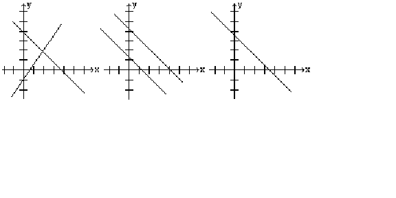
Determine the linear systems that have no solution.
Solve the linear systems that have infinitely many solutions.

If we consider the intersection of two lines in a plane, three things can happen.

The lines intersect in exactly one point. This is called an independent system.
The lines are parallel, so they do not intersect. This is called an inconsistent system.
The lines coincide, so they intersect at infinitely many points. This is a dependent system.

The figures below shows all three cases.

The graph on the right depicts an independent system. The graph in the middle depicts an inconsistent system. The graph on the left depicts a dependent system. — **Figure 2.1**

Every system of equations has either one solution, no solution, or infinitely many solutions.

In the, we used the Gauss-Jordan method to solve systems that had exactly one solution. In this section, we will determine the systems that have no solution, and solve the systems that have infinitely many solutions.

Example 19

Solve the following system of equations.

$x + y = 7$

$x + y = 9$

Let us use the Gauss-Jordan method to solve this system. The augmented matrix is as follows.

$[\begin{matrix} 1 & 1 & ∣ & 7 \\ 1 & 1 & ∣ & 9 \end{matrix}] [\begin{matrix} x + y = 7 \\ x + y = 9 \end{matrix}]$

If we multiply the first row by – 1 and add to the second row, we get

$[\begin{matrix} 1 & 1 & ∣ & 7 \\ 0 & 0 & ∣ & 2 \end{matrix}] [\begin{matrix} x + y = 7 \\ 0x + 0y = 2 \end{matrix}]$

Since 0 cannot equal 2, the last equation cannot be true for any choices of $x$ and $y$ .

Alternatively, it is clear that the two lines are parallel; therefore, they do not intersect.

At this stage, we are going to start using a calculator to row reduce the augmented matrix.

Example 21

Solve the following system of equations.

$x + y = 7$

The problem clearly asks for the intersection of two lines that are the same; that is, the lines coincide. This means the lines intersect at an infinite number of points.

A few intersection points are listed as follows: (3, 4), (5, 2), (–1, 8), (–6, 13) etc. However, when a system has an infinite number of solutions, the solution is often expressed in the parametric form. This can be accomplished by assigning an arbitrary constant, $t$ , to one of the variables, and then solving for the remaining variables. Therefore, if we let $y = t$ , then $x = 7 - t$ . Or we can say all ordered pairs of the form ( $7 minus t$ , $t$ ) satisfy the given system of equations.

Alternatively, while solving the Gauss-Jordan method, we will get the reduced row-echelon form given below.

$open bracket 1, 1, ∣, 7; 0, 0, ∣, 0 close bracket$

The row of all zeros, can simply be discarded in a manner that it never existed. This leaves us with only one equation but two variables. And whenever there are more variables than the equations, the solution must be expressed in terms of an arbitrary constant, as above. That is, $x = 7 - t$ , $y = t$ .

Example 22

Solve the following system of equations.

$x + y + z = 2$

$2x + y - z = 3$

$3x + 2y = 5$

The augmented matrix and the reduced row-echelon form are given below.

$open bracket 1, 1, 1, ∣, 2; 2, 1, minus 1, ∣, 3; 3, 2, 0, ∣, 5 close bracket$

$open bracket 1, 0, minus 2, ∣, 1; 0, 1, 3, ∣, 1; 0, 0, 0, ∣, 0 close bracket$

Since the last equation dropped out, we are left with two equations and three variables. This means the system has infinite number of solutions. We express those solutions in the parametric form by letting the last variable $z$ equal the parameter $t$ .

The first equation reads $x - 2z = 1$ , therefore, $x = 1 + 2z$ .

The second equation reads $y + 3z = 1$ , therefore, $y = 1 - 3z$ .

And now if we let $z = t$ , the solution is expressed as follows:

$x = 1 + 2t, y = 1 - 3t, z = t .$

The reader should note that particular solutions to the system can be obtained by assigning values to the parameter $t$ . For example, if we let $t equals 2$ , we have the solution (5, –5, 2).

Example 23

Solve the following system of equations.

$x + 2y - 3z = 5$

$2x + 4y - 6z = 10$

$3x + 6y - 9z = 15$

The reduced row-echelon form is given below.

$open bracket 1, 2, minus 3, ∣, 5; 0, 0, 0, ∣, 0; 0, 0, 0, ∣, 0 close bracket$

This time the last two equations drop out, and we are left with one equation and three variables. Again, there are infinite number of solutions. But this time the answer must be expressed in terms of two arbitrary constants.

If we let $z = t$ and let $y = s$ , then the first equation $x + 2y - 3z = 5$ results in $x = 5 - 2s + 3t$ .

We rewrite the solution as: $x = 5 - 2s + 3t$ , $y = s$ , $z = t$ .

We summarize our discussion in the following table.

If any row of the reduced row-echelon form of the matrix gives a false statement such as 0 = 1, the system is inconsistent and has no solution.
If the reduced row echelon form has fewer equations than the variables and the system is consistent, then the system has an infinite number of solutions. Remember the rows that contain all zeros are dropped.
1. If a system has an infinite number of solutions, the solution must be expressed in the parametric form.
2. The number of arbitrary parameters equals the number of variables minus the number of equations.

Inverse Matrices

Section Overview

In this section you will learn to:

Find the inverse of a matrix, if it exists.
Use inverses to solve linear systems.

In this section, we will learn to find the inverse of a matrix, if it exists. Later, we will use matrix inverses to solve linear systems.

Definition of an Inverse: An $n \times n$ matrix has an inverse if there exists a matrix $B$ such that $AB = BA = I_{n}$ , where $I_{n}$ is an $n \times n$ identity matrix. The inverse of a matrix $A$ , if it exists, is denoted by the symbol $A^{- 1}$ .

Example 24

Given matrices $A$ and $B$ below, verify that they are inverses.

$A = [\begin{matrix} 4 & 1 \\ 3 & 1 \end{matrix}] B = [\begin{matrix} 1 & - 1 \\ - 3 & 4 \end{matrix}]$

The matrices are inverses if the product $AB$ and $BA$ both equal $I sub 2$ , the identity matrix of dimension $2 times 2$ .

$AB = [\begin{matrix} 4 & 1 \\ 3 & 1 \end{matrix}] [\begin{matrix} 1 & - 1 \\ - 3 & 4 \end{matrix}] = [\begin{matrix} 1 & 0 \\ 0 & 1 \end{matrix}] and BA = [\begin{matrix} 1 & - 1 \\ - 3 & 4 \end{matrix}] [\begin{matrix} 4 & 1 \\ 3 & 1 \end{matrix}] = [\begin{matrix} 1 & 0 \\ 0 & 1 \end{matrix}]$

Clearly that is the case; therefore, the matrices A and B are inverses of each other.

Example 25

Find the inverse of the following matrix.

$A equals open bracket 3, 1; 5, 2 close bracket$

Suppose $A$ has an inverse, and it is

$B = [\begin{matrix} a & b \\ c & d \end{matrix}]$

Then $A B = I$

$open bracket 3, 1; 5, 2 close bracket open bracket a, b; c, d close bracket equals open bracket 1, 0; 0, 1 close bracket$

After multiplying the two matrices on the left side, we get

$[\begin{matrix} 3a + c & 3b + 6 \\ 5a + 2c & 5b + 2d \end{matrix}] = [\begin{matrix} 1 & 0 \\ 0 & 1 \end{matrix}]$

Equating the corresponding entries, we get four equations with four unknowns as follows:

$3a + c = 1 3b + d = 0$

$5a + 2c = 0 5b + 2d = 1$

Solving this system, we get

$a = 2 b = - 1 c = - 5 d = 3$

Therefore, the inverse of the matrix $A$ is

$[\begin{matrix} 2 & - 1 \\ - 5 & 3 \end{matrix}]$

In this problem, finding the inverse of matrix $A$ amounted to solving the system of equations:

$3a + c = 1 3b + d = 0$

$5a + 2c = 0 5b + 2d = 1$

Actually, it can be written as two systems, one with variables $a$ and $c$ , and the other with $b$ and $d$ . The augmented matrices for both are given below.

$open bracket 3, 1, ∣, 1; 5, 2, ∣, 0 close bracket and open bracket 3, 1, ∣, 0; 5, 2, ∣, 1 close bracket$

As we look at the two augmented matrices, we notice that the coefficient matrix for both the matrices is the same. Which implies the row operations of the Gauss-Jordan method will also be the same. A great deal of work can be saved if the two right hand columns are grouped together to form one augmented matrix as below.

$open bracket 3, 1, ∣, 1, 0; 5, 2, ∣, 0, 1 close bracket$

And solving this system, we get

$[\begin{matrix} 1 & 0 & ∣ & 2 & - 1 \\ 0 & 1 & ∣ & - 5 & 3 \end{matrix}]$

The matrix on the right side of the vertical line is the $A^{- 1}$ matrix.

What you just witnessed is no coincidence. This is the method that is often employed in finding the inverse of a matrix.

We list the steps, as follows:

Example 27

Given the matrix $A$ below, find its inverse.

$A = [\begin{matrix} 1 & - 1 & 1 \\ 2 & 3 & 0 \\ 0 & - 2 & 1 \end{matrix}]$

We write the augmented matrix as follows.

$[\begin{matrix} 1 & - 1 & 1 & ∣ & 1 & 0 & 0 \\ 2 & 3 & 0 & ∣ & 0 & 1 & 0 \\ 0 & - 2 & 1 & ∣ & 0 & 0 & 1 \end{matrix}]$

We reduce this matrix using the Gauss-Jordan method.

Multiplying the first row by –2 and adding it to the second row, we get

$[\begin{matrix} 1 & - 1 & 1 & ∣ & 1 & 0 & 0 \\ 0 & 5 & - 2 & ∣ & - 2 & 1 & 0 \\ 0 & - 2 & 1 & ∣ & 0 & 0 & 1 \end{matrix}]$

If we swap the second and third rows, we get

$[\begin{matrix} 1 & - 1 & 1 & ∣ & 1 & 0 & 0 \\ 0 & - 2 & 1 & ∣ & 0 & 0 & 1 \\ 0 & 5 & - 2 & ∣ & - 2 & 1 & 0 \end{matrix}]$

Divide the second row by –2. The result is

$[\begin{matrix} 1 & - 1 & 1 & ∣ & 1 & 0 & 0 \\ 0 & 1 & - 1 / 2 & ∣ & 0 & 0 & - 1 / 2 \\ 0 & 5 & - 2 & ∣ & - 2 & 1 & 0 \end{matrix}]$

Let us do two operations here. 1) Add the second row to first, 2) Add -5 times the second row to the third. And we get

$[\begin{matrix} 1 & 0 & 1 / 2 & ∣ & 1 & 0 & - 1 / 2 \\ 0 & 1 & - 1 / 2 & ∣ & 0 & 0 & - 1 / 2 \\ 0 & 0 & 1 / 2 & ∣ & - 2 & 1 & 5 / 2 \end{matrix}]$

Multiplication of the third row by 2 results in

$[\begin{matrix} 1 & 0 & 1 / 2 & ∣ & 1 & 0 & - 1 / 2 \\ 0 & 1 & - 1 / 2 & ∣ & 0 & 0 & - 1 / 2 \\ 0 & 0 & 1 & ∣ & - 4 & 2 & 5 \end{matrix}]$

Multiply the third row by $1 / 2$ and add it to the second. Also, multiply the third row by $minus 1 / 2$ and add it to the first. We get

$[\begin{matrix} 1 & 0 & 0 & ∣ & 3 & - 1 & - 3 \\ 0 & 1 & 0 & ∣ & - 2 & 1 & 2 \\ 0 & 0 & 1 & ∣ & - 4 & 2 & 5 \end{matrix}]$

Therefore, the inverse of matrix $A$ is

$[\begin{matrix} 3 & - 1 & - 3 \\ - 2 & 1 & 2 \\ - 4 & 2 & 5 \end{matrix}]$

One should verify the result by multiplying the two matrices to see if the product does, indeed, equal the identity matrix.

Now that we know how to find the inverse of a matrix, we will use inverses to solve systems of equations. The method is analogous to solving a simple equation like the one below.

$\frac{2}{3} x = 4$

To solve a linear system, we first write the system in the matrix equation $AX = B$ , where $A$ is the coefficient matrix, $X$ the matrix of variables, and $B$ the matrix of constant terms. We then multiply both sides of this equation by the multiplicative inverse of the matrix $A$ .

Consider the following example.

Example 29

Solve the following system

$3x + y = 3$

$5x + 2y = 4$

To solve the above equation, first we express the system as

$AX = B$

where $A$ is the coefficient matrix, and $B$ is the matrix of constant terms. We get

$open bracket 3, 1; 5, 2 close bracket open bracket x; y close bracket equals open bracket 3; 4 close bracket$

To solve this system, we multiply both sides of the matrix equation $AX = B$ by $A^{- 1}$ . Since the matrix $A$ is the same matrix $A$ whose inverse we found in Example 25,

$A^{- 1} = [\begin{matrix} 2 & - 1 \\ - 5 & 3 \end{matrix}]$

Multiplying both sides by $A^{- 1}$ , we get

$[\begin{matrix} 2 & - 1 \\ - 5 & 3 \end{matrix}] [\begin{matrix} 3 & 1 \\ 5 & 2 \end{matrix}] [\begin{matrix} x \\ y \end{matrix}] = [\begin{matrix} 2 & - 1 \\ - 5 & 3 \end{matrix}] [\begin{matrix} 3 \\ 4 \end{matrix}]$

$[\begin{matrix} 1 & 0 \\ 0 & 1 \end{matrix}] [\begin{matrix} x \\ y \end{matrix}] = [\begin{matrix} 2 \\ - 3 \end{matrix}]$

$[\begin{matrix} x \\ y \end{matrix}] = [\begin{matrix} 2 \\ - 3 \end{matrix}]$

Therefore, $x equals 2$ , and $y = - 3$ .

Example 30

Solve the following system

$x - y + z = 6$

$2x + 3y = 1$

$- 2y + z = 5$

To solve the above equation, we write the system in the matrix form $AX = B$ as follows:

$[\begin{matrix} 1 & - 1 & 1 \\ 2 & 3 & 0 \\ 0 & - 2 & 1 \end{matrix}] [\begin{matrix} x \\ y \\ z \end{matrix}] = [\begin{matrix} 6 \\ 1 \\ 5 \end{matrix}]$

To solve this system, we need inverse of $A$ . From Example 27, we have

$A^{- 1} = [\begin{matrix} 3 & - 1 & - 3 \\ - 2 & 1 & 2 \\ - 4 & 2 & 5 \end{matrix}]$

We multiply both sides of the matrix equation $AX = B$ , by $A^{- 1}$ , we get

$[\begin{matrix} 3 & - 1 & - 3 \\ - 2 & 1 & 2 \\ - 4 & 2 & 5 \end{matrix}] [\begin{matrix} 1 & - 1 & - 3 \\ 2 & 3 & 0 \\ 0 & - 2 & 1 \end{matrix}] [\begin{matrix} x \\ y \\ z \end{matrix}] = [\begin{matrix} 3 & - 1 & - 3 \\ - 2 & 1 & 2 \\ - 4 & 2 & 5 \end{matrix}] [\begin{matrix} 6 \\ 1 \\ 5 \end{matrix}]$

After multiplying the matrices, we get

$[\begin{matrix} 1 & 0 & 0 \\ 0 & 1 & 0 \\ 0 & 0 & 1 \end{matrix}] [\begin{matrix} x \\ y \\ z \end{matrix}] = [\begin{matrix} 2 \\ - 1 \\ 3 \end{matrix}]$

$[\begin{matrix} x \\ y \\ z \end{matrix}] = [\begin{matrix} 2 \\ - 1 \\ 3 \end{matrix}]$

Once again, we remind the reader that not every system of equations can be solved by the matrix inverse method. Although the Gauss-Jordan method works for every situation, the matrix inverse method works only in cases where the inverse of the square matrix exists. In such cases the system has a unique solution.

We summarize our discussion in the following table.

Write the augmented matrix $open bracket A, ∣, I sub n close bracket$ .
Write the augmented matrix in step 1 in reduced row echelon form.
If the reduced row echelon form in 2 is $open bracket I sub n, ∣, B close bracket$ , then $B$ is the inverse of $A$ .
If the left side of the row reduced echelon is not an identity matrix, the inverse does not exist.

Express the system in the matrix equation $AX = B$ .
To solve the equation $AX = B$ , we multiply on both sides by $A^{- 1}$ .

Application of Matrices in Cryptography

In this section, we see a use of matrices in encoding and decoding secret messages. There are many techniques used, but we will use a method that first converts the secret message into a string of numbers by arbitrarily assigning a number to each letter of the message. Next we convert this string of numbers into a new set of numbers by multiplying the string by a square matrix of our choice that has an inverse. This new set of numbers represents the coded message. To decode the message, we take the string of coded numbers and multiply it by the inverse of the matrix to get the original string of numbers. Finally, by associating the numbers with their corresponding letters, we obtain the original message.

In this section, we will use the correspondence where the letters A to Z correspond to the numbers 1 to 26, as shown below, and a space is represented by the number 27, and all punctuation is ignored.

**Table 2.2**
A	B	C	D	E	F	G	H	I	J	K	L	M
1	2	3	4	5	6	7	8	9	10	11	12	13
N	O	P	Q	R	S	T	U	V	W	X	Y	Z
14	15	16	17	18	19	20	21	22	23	24	25	26

Example 31

Use the matrix $A equals open bracket 1, 2; 1, 3 close bracket$ to encode the message: ATTACK NOW!

We divide the letters of the message into groups of two.

AT TA CK –N OW

We assign the numbers to these letters from the above table, and convert each pair of numbers into $2 times 1$ matrices. In the case where a single letter is left over on the end, a space is added to make it into a pair.

$[\begin{matrix} A \\ T \end{matrix}] = [\begin{matrix} 1 \\ 20 \end{matrix}] [\begin{matrix} T \\ A \end{matrix}] = [\begin{matrix} 20 \\ 1 \end{matrix}] [\begin{matrix} C \\ K \end{matrix}] = [\begin{matrix} 3 \\ 11 \end{matrix}] [\begin{matrix} _ \\ N \end{matrix}] = [\begin{matrix} 27 \\ 14 \end{matrix}] [\begin{matrix} O \\ W \end{matrix}] = [\begin{matrix} 15 \\ 23 \end{matrix}]$

So at this stage, our message expressed as $2 times 1$ matrices is as follows.

$open bracket 1; 20 close bracket open bracket 20; 1 close bracket open bracket 3; 11 close bracket open bracket 27; 14 close bracket open bracket 15; 23 close bracket$

Now to encode, we multiply, on the left, each matrix of our message by the matrix A. For example, the product of A with our first matrix is

$open bracket 1, 2; 1, 3 close bracket open bracket 1; 20 close bracket equals open bracket 41; 61 close bracket$

By multiplying each of the matrices in ( I ) by the matrix A, we get the desired coded message given below.

$open bracket 41; 61 close bracket open bracket 22; 23 close bracket open bracket 25; 36 close bracket open bracket 55; 69 close bracket open bracket 61; 84 close bracket$

Example 32

Decode the following message that was encoded using matrix $A equals open bracket 1, 2; 1, 3 close bracket$ .

$open bracket 21; 26 close bracket open bracket 37; 53 close bracket open bracket 45; 54 close bracket open bracket 74; 101 close bracket open bracket 53; 69 close bracket$

Since this message was encoded by multiplying by the matrix A in Example 31, we decode this message by first multiplying each matrix, on the left, by the inverse of matrix A given below.

$A^{- 1} = [\begin{matrix} 3 & - 2 \\ - 1 & 1 \end{matrix}]$

For example,

$[\begin{matrix} 3 & - 2 \\ - 1 & 1 \end{matrix}] [\begin{matrix} 21 \\ 26 \end{matrix}] = [\begin{matrix} 11 \\ 5 \end{matrix}]$

By multiplying each of the matrices in ( II ) by the matrix $A^{- 1}$ , we get the following.

$open bracket 11; 5 close bracket open bracket 5; 16 close bracket open bracket 27; 9 close bracket open bracket 20; 27 close bracket open bracket 21; 16 close bracket$

Finally, by associating the numbers with their corresponding letters, we obtain the following.

$open bracket K; E close bracket open bracket E; P close bracket open bracket _; I close bracket open bracket T; _ close bracket open bracket U; P close bracket$

And the message reads: KEEP IT UP.

Now suppose we wanted to use a $3 times 3$ matrix to encode a message, then instead of dividing the letters into groups of two, we would divide them into groups of three.

Example 33

Using the matrix $B = [\begin{matrix} 1 & 1 & - 1 \\ 1 & 0 & 1 \\ 2 & 1 & 1 \end{matrix}]$ , encode the message: ATTACK NOW!

We divide the letters of the message into groups of three.

ATT ACK –NO W––

Note that since the single letter "W" was left over on the end, we added two spaces to make it into a triplet.

Now we assign the numbers their corresponding letters from the table, and convert each triplet of numbers into $3 times 1$ matrices. We get

$[\begin{matrix} A \\ T \\ T \end{matrix}] = [\begin{matrix} 1 \\ 20 \\ 20 \end{matrix}] [\begin{matrix} A \\ C \\ K \end{matrix}] = [\begin{matrix} 1 \\ 3 \\ 11 \end{matrix}] [\begin{matrix} _ \\ N \\ O \end{matrix}] = [\begin{matrix} 27 \\ 14 \\ 15 \end{matrix}] [\begin{matrix} W \\ _ \\ _ \end{matrix}] = [\begin{matrix} 23 \\ 27 \\ 27 \end{matrix}]$

So far we have,

$open bracket 1; 20; 20 close bracket open bracket 1; 3; 11 close bracket open bracket 27; 14; 15 close bracket open bracket 23; 27; 27 close bracket$

We multiply, on the left, each matrix of our message by the matrix B. For example,

$[\begin{matrix} 1 & 1 & - 1 \\ 1 & 0 & 1 \\ 2 & 1 & 1 \end{matrix}] [\begin{matrix} 1 \\ 20 \\ 20 \end{matrix}] = [\begin{matrix} 1 \\ 21 \\ 42 \end{matrix}]$

By multiplying each of the matrices in ( III ) by the matrix B, we get the desired coded message as follows:

$open bracket 1; 21; 42 close bracket open bracket minus 7; 12; 16 close bracket open bracket 26; 42; 83 close bracket open bracket 23; 50; 100 close bracket$

If we need to decode this message, we simply multiply the coded message by $B^{- 1}$ , and associate the numbers with the corresponding letters of the alphabet.

Example 34

Decode the following message that was encoded using matrix $B = [\begin{matrix} 1 & 1 & - 1 \\ 1 & 0 & 1 \\ 2 & 1 & 1 \end{matrix}]$ .

$open bracket 11; 20; 43 close bracket open bracket 25; 10; 41 close bracket open bracket 22; 14; 14 close bracket$

Since this message was encoded by multiplying by the matrix B. We first determine inverse of B.

$B^{- 1} = [\begin{matrix} 1 & 2 & - 1 \\ - 1 & - 3 & 2 \\ - 1 & - 1 & 1 \end{matrix}]$

To decode the message, we multiply each matrix, on the left, by $B^{- 1}$ . For example,

$[\begin{matrix} 1 & 2 & - 1 \\ - 1 & - 3 & 2 \\ - 1 & - 1 & 1 \end{matrix}] [\begin{matrix} 11 \\ 20 \\ 43 \end{matrix}] = [\begin{matrix} 8 \\ 15 \\ 12 \end{matrix}]$

By multiplying each of the matrices in ( IV ) by the matrix $B^{- 1}$ , we get the following.

$open bracket 8; 15; 12 close bracket open bracket 4; 27; 6 close bracket open bracket 9; 18; 5 close bracket$

Finally, by associating the numbers with their corresponding letters, we obtain the following.

$[\begin{matrix} H \\ O \\ L \end{matrix}] [\begin{matrix} D \\ F \end{matrix}] [\begin{matrix} I \\ R \\ E \end{matrix}]$

And the message reads: HOLD FIRE.

We summarize.

Applications – Leontief Models

In the 1930's, Wassily Leontief used matrices to model economic systems. His models, often referred to as the input-output models, divide the economy into sectors where each sector produces goods and services not only for itself but also for other sectors. These sectors are dependent on each other and the total input always equals the total output. In 1973, he won the Nobel Prize in Economics for his work in this field. In this section we look at both the closed and the open models that he developed.

The Closed Model As an example of the closed model, we look at a very simple economy, where there are only three sectors: food, shelter, and clothing.

Example 36

We assume that in a village there is a farmer, carpenter, and a tailor, who provide the three essential goods: food, shelter, and clothing. Suppose the farmer himself consumes 40% of the food he produces, and gives 40% to the carpenter, and 20% to the tailor. Thirty percent of the carpenter's production is consumed by himself, 40% by the farmer, and 30% by the carpenter. Fifty percent of the tailor's production is used by himself, 30% by the farmer, and 20% by the tailor. Write the matrix that describes this closed model.

The table below describes the above information.

**Table 2.3**
	The proportion produced by the farmer	The propotion produced by the carpenter	The proportion produced by the tailor
The proportion used by the farmer	.40	.40	.30
The proportion used by the carpenter	.40	.30	.20
The proportion used by the tailor	.20	.30	.50

In a matrix form it can be written as follows.

$A equals open bracket .40, .40, .30; .40, .30, .20; .20, .30, .50 close bracket$

This matrix is called the input-output matrix. It is important that we read the matrix correctly. For example the entry $A sub 23$ , the entry in row 2 and column 3, represents the following.

$A sub 23 equals 20 %$ of the tailor's production is used by the carpenter.

$A sub 33 equals 50 %$ of the tailor's production is used by the tailor.

Example 37

In Example 36 above, how much should each person get for his efforts?

We choose the following variables.

$x = Farmer's pay$

$y = Carpenter's pay$

$z = Tailor's pay$

As we said earlier, in this model input must equal output. That is, the amount paid by each equals the amount received by each.

Let us say the farmer gets paid $x$ dollars. Let us now look at the farmer's expenses. The farmer uses up 40% of his own production, that is, of the $x$ dollars he gets paid, he pays himself $.40 x$ dollars, he pays $.40 y$ dollars to the carpenter, and $.30 z$ to the tailor. Since the expenses equal the wages, we get the following equation.

$x = . 40 x + . 40 y + . 30 z$

In the same manner, we get

$y = . 40 x + . 30 y + . 20 z$

$z = . 20 x + . 30 y + . 50 z$

The above system can be written as

$open bracket x; y; z close bracket equals open bracket .40, .40, .30; .40, .30, .20; .20, .30, .50 close bracket open bracket x; y; z close bracket$

This system is often referred to as

$X = AX$

Simplification results in

$. 60 x - . 40 y - . 30 z = 0$

$- . 40 x + . 70 y - . 20 z = 0$

$- . 20 x - . 30 y + . 50 z = 0$

Solving for $x$ , $y$ , and $z$ using the Gauss-Jordan method, we get

$x = \frac{29}{26} t y = \frac{12}{13} t and z = t$

Since we are only trying to determine the proportions of the pay, we can choose t to be any value. Suppose we let $t equals $ 2600$ , then we get

$x = $ 2900 y = $ 2400 and z = $ 2600$

The Open Model

The open model is more realistic, as it deals with the economy where sectors of the economy not only satisfy each others needs, but they also satisfy some outside demands. In this case, the outside demands are put on by the consumer. But the basic assumption is still the same; that is, whatever is produced is consumed.

Let us again look at a very simple scenario. Suppose the economy consists of three people, the farmer $F$ , the carpenter $C$ , and the tailor $T$ . A part of the farmer's production is used by all three, and the rest is used by the consumer. In the same manner, a part of the carpenter's and the tailor's production is used by all three, and rest is used by the consumer.

Let us assume that whatever the farmer produces, 20% is used by him, 15% by the carpenter, 10% by the tailor, and the consumer uses the other 40 billion dollars worth of the food. Ten percent of the carpenter's production is used by him, 25% by the farmer, 5% by the tailor, and 50 billion dollars worth by the consumer. Fifteen percent of the clothing is used by the tailor, 10% by the farmer, 5% by the carpenter, and the remaining 60 billion dollars worth by the consumer. We write the internal consumption in the following table, and express the demand as the matrix D.

**Table 2.4**
	$F$ produces	$C$ produces	$T$ produces
$F$ uses	.20	.25	.10
$C$ uses	.15	.10	.05
$T$ uses	.10	.05	.15

The consumer demand for each industry in billions of dollars is given below.

$D equals open bracket 40; 50; 60 close bracket$

Example 38

In Example 37, what should be, in billions of dollars, the required output by each industry to meet the demand given by the matrix D?

We choose the following variables.

$x = Farmer's output$

$y = Carpenter's output$

$z = Tailor's output$

In the closed model, our equation was $X = AX$ , that is, the total input equals the total output. This time our equation is similar with the exception of the demand by the consumer.

So our equation for the open model should be $X = AX + D$ , where $D$ represents the demand matrix. We express it as follows:

$X = AX + D$

$[\begin{matrix} x \\ y \\ z \end{matrix}] = [\begin{matrix} . 20 & . 25 & . 10 \\ . 15 & . 10 & . 05 \\ . 10 & . 05 & . 15 \end{matrix}] [\begin{matrix} x \\ y \\ z \end{matrix}] + [\begin{matrix} 40 \\ 50 \\ 60 \end{matrix}]$

To solve this system, we write it as

$X = AX + D$

$(I - A) X = D$

where I is a 3 by 3 identity matrix

$X = {(I - A)}^{- 1} D$

$I - A = [\begin{matrix} . 80 & - . 25 & - . 10 \\ - . 15 & . 90 & - . 05 \\ - . 10 & - . 05 & . 85 \end{matrix}]$

${(I - A)}^{- 1} = [\begin{matrix} 1.3445 & . 3835 & . 1807 \\ . 2336 & 1.1814 & . 097 \\ . 1719 & . 1146 & 1.2034 \end{matrix}]$

$X equals open bracket 1.3445, .3835, .1807; .2336, 1.1814, .097; .1719, .1146, 1.2034 close bracket open bracket 40; 50; 60 close bracket$

$X equals open bracket 83.7999; 74.2341; 84.8138 close bracket$

Therefore, the three industries must produce the following amount of goods in billions of dollars.

$Farmer = $ 83.7999 Carpenter = $ 74.2341 Tailor = $ 84.813$

We will do one more problem like the one above, except this time we give the amount of internal and external consumption in dollars and ask for the proportion of the amounts consumed by each of the industries. In other words, we ask for the matrix A.

Example 39

Suppose an economy consists of three industries $F$ , $C$ , and $T$ . Again, each of the industries produces for internal consumption among themselves, as well as, the external demand by the consumer. The following table gives information about the use of each industry's production in dollars.

**Table 2.5**
	$F$	$C$	$T$	Demand	Total
$F$	40	50	60	100	250
$C$	30	40	40	110	220
$T$	20	30	30	120	200

The first row says that of the $250 dollars worth of production by the industry $F$ , $40 is used by $F$ , $50 is used by $C$ , $60 is used by $T$ , and the remainder of $100 is used by the consumer. The other rows are described in a similar manner.

Find the proportion of the amounts consumed by each of the industries. In other words, find the matrix A.

Once again, the total input equals the total output.

We are being asked to determine the following:

How much of the production of each of the three industries, $F$ , $C$ , and $T$ is required to produce one unit of $F$ ? In the same way, how much of the production of each of the three industries, $F$ , $C$ , and $T$ is required to produce one unit of $C$ ? And finally, how much of the production of each of the three industries, $F$ , $C$ , and $T$ is required to produce one unit of $T$ ?

Since we are looking for proportions, we need to divide the production of each industry by the total production for each industry.

We analyze as follows:

To produce 250 units of $F$ , we need to use 40 units of $F$ , 30 units of $C$ , and 20 units of $T$ .

Therefore, to produce 1 unit of $F$ , we need to use 40/250 units of $F$ , 30/250 units of $C$ , and 20/250 units of $T$ .

To produce 220 units of $C$ , we need to use 50 units of $F$ , 40 units of $C$ , and 30 units of $T$ .

Therefore, to produce 1 unit of $C$ , we need to use 50/220 units of $F$ , 40/220 units of $C$ , and 30/220 units of $T$ .

To produce 200 units of $T$ , we need to use 60 units of $F$ , 40 units of $C$ , and 30 units of $T$ .

Therefore, to produce 1 unit of $T$ , we need to use 60/200 units of $F$ , 40/200 units of $C$ , and 30/200 units of $T$ .

We obtain the following matrix.

$A equals open bracket 40 / 250, 50 / 220, 60 / 200; 30 / 250, 40 / 220, 40 / 220; 20 / 250, 30 / 220, 30 / 220 close bracket$

$A equals open bracket .1600, .2273, .3000; .1200, .1818, .2000; .0800, .1364, .1500 close bracket$

Clearly

$AX + D = X$

$[\begin{matrix} 40 / 250 & 50 / 220 & 60 / 200 \\ 30 / 250 & 40 / 220 & 40 / 200 \\ 20 / 250 & 30 / 220 & 30 / 200 \end{matrix}] [\begin{matrix} 250 \\ 220 \\ 200 \end{matrix}] + [\begin{matrix} 100 \\ 110 \\ 120 \end{matrix}] = [\begin{matrix} 250 \\ 220 \\ 200 \end{matrix}]$

We summarize as follows:

Example 40 LEONTIEF'S MODELS

All consumption is within the industries. There is no external demand.
$Input = Output$
$X = AX$ or $(I - A) X = 0$

In addition to internal consumption, there is an outside demand by the consumer.
$Input = Output$
$X = AX + D$ or $X = {(I - A)}^{- 1} D$

Adapted from Applied Finite Mathematics by Rupinder Sekhon (De Anza College), originally published by OpenStax CNX (cnx.org, collection col10613), licensed under CC BY 3.0. Changes were made. License: CC-BY-3.0.