6.6 Simulating data for t-tests

An “advanced” topic for $t$ -tests is the idea of using R to conduct simulations for $t$ -tests.

If you recall, $t$ is a property of a sample. We calculate $t$ from our sample. The $t$ distribution is the hypothetical behavior of our sample. That is, if we had taken thousands upon thousands of samples, and calculated $t$ for each one, and then looked at the distribution of those $t$ ’s, we would have the sampling distribution of $t$ !

It can be very useful to get in the habit of using R to simulate data under certain conditions, to see how your sample data, and things like $t$ behave. Why is this useful? It mainly prepares you with some intuitions about how sampling error (random chance) can influence your results, given specific parameters of your design, such as sample-size, the size of the mean difference you expect to find in your data, and the amount of variation you might find. These methods can be used formally to conduct power-analyses. Or more informally for data sense.

6.6.1 Simulating a one-sample t-test

Here are the steps you might follow to simulate data for a one sample $t$ -test.

Make some assumptions about what your sample (that you might be planning to collect) might look like. For example, you might be planning to collect 30 subjects worth of data. The scores of those data points might come from a normal distribution (mean = 50, sd = 10).
sample simulated numbers from the distribution, then conduct a $t$ -test on the simulated numbers. Save the statistics you want (such as $t$ s and $p$ s), and then see how things behave.

Let’s do this a couple different times. First, let’s simulate samples with N = 30, taken from a normal (mean= 50, sd = 25). We’ll do a simulation with 1000 simulations. For each simulation, we will compare the sample mean with a population mean of 50. There should be no difference on average here. Figure 6.11 is the null distribution that we are simulating.

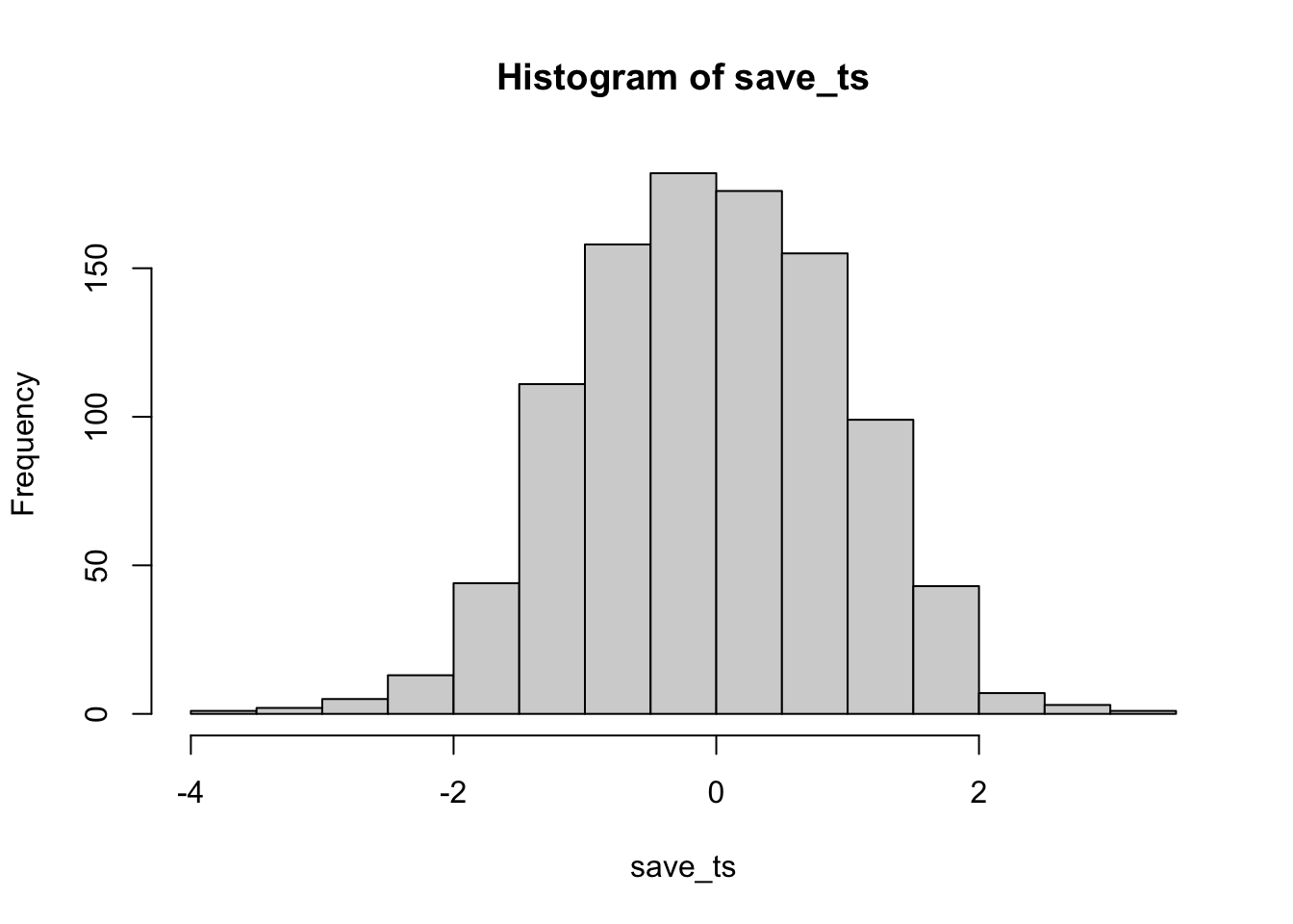
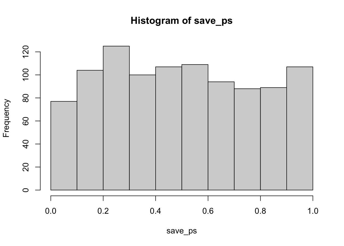
Histogram of t-values from 1,000 simulated experiments in which the null hypothesis is true. The values form a symmetric bell shape centered on zero, with most falling between -2 and 2 and only a handful beyond those points. — Figure 6.11: The distribution of $t$ -values under the null. These are the $t$ values that are produced by chance alone.

Histogram of 1,000 simulated p-values from null t-tests, spanning 0 to 1. The ten bars are all roughly equal height, about 80 to 125 simulations each, showing that p-values are spread approximately uniformly when there is no true effect. — Figure 6.12: The distribution of $p$ -values that are observed is flat under the null.

Neat. We see both a $t$ distribution, that looks like $t$ distribution as it should. And we see the $p$ distribution. This shows us how often we get $t$ values of particular sizes. You may find it interesting that the $p$ -distribution is flat under the null, which we are simulating here. This means that you have the same chances of a getting a $t$ with a p-value between 0 and 0.05, as you would for getting a $t$ with a p-value between.90 and.95. Those ranges are both ranges of 5%, so there are an equal amount of $t$ values in them by definition.

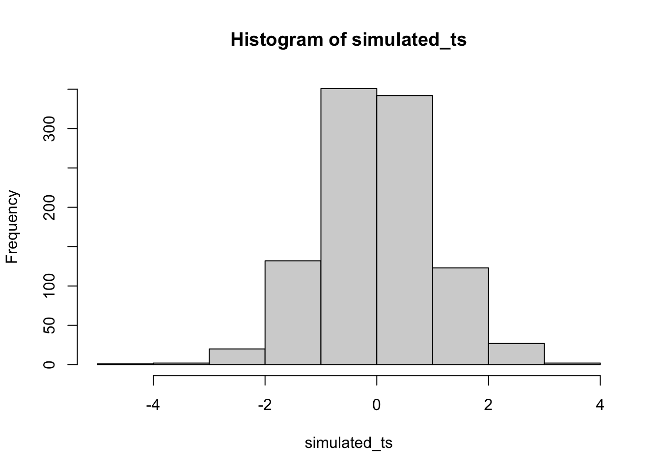
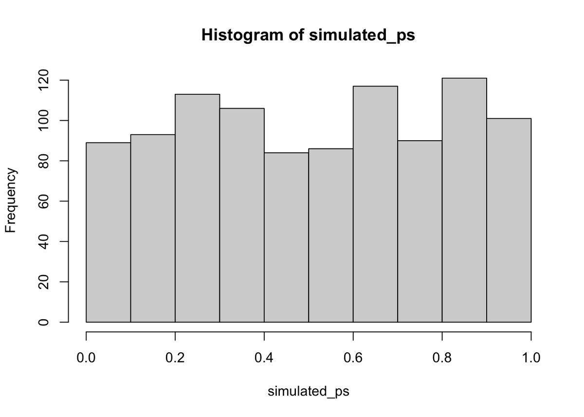
Here’s another way to do the same simulation in R, using the replicate function, instead a for loop:

Histogram of 1,000 t-values generated by one line of R code that repeatedly t-tests random normal samples (n=30, mean 50) against mu=50. The values form a symmetric bell centered on zero, with nearly all between -3 and 3. — Figure 6.13: Simulating $t$ s in R.

Histogram of 1,000 p-values produced by a single line of R code that repeatedly t-tests random normal samples with no true effect. The bars are roughly level across the whole 0-to-1 range, illustrating the flat p-value distribution expected under the null. — Figure 6.14: Simulating $p$ s in R.

6.6.2 Simulating a paired samples t-test

The code below is set up to sample 10 scores for condition A and B from the same normal distribution. The simulation is conducted 1000 times, and the $t$ s and $p$ s are saved and plotted for each.

save_ps <- length(1000)
save_ts <- length(1000)
for ( i in 1:1000 ){
  condition_A <- rnorm(10,10,5)
  condition_B <- rnorm(10,10,5)
  differences <- condition_A - condition_B
  t_test <- t.test(differences, mu=0)
  save_ps[i] <- t_test$p.value
  save_ts[i] <- t_test$statistic
}

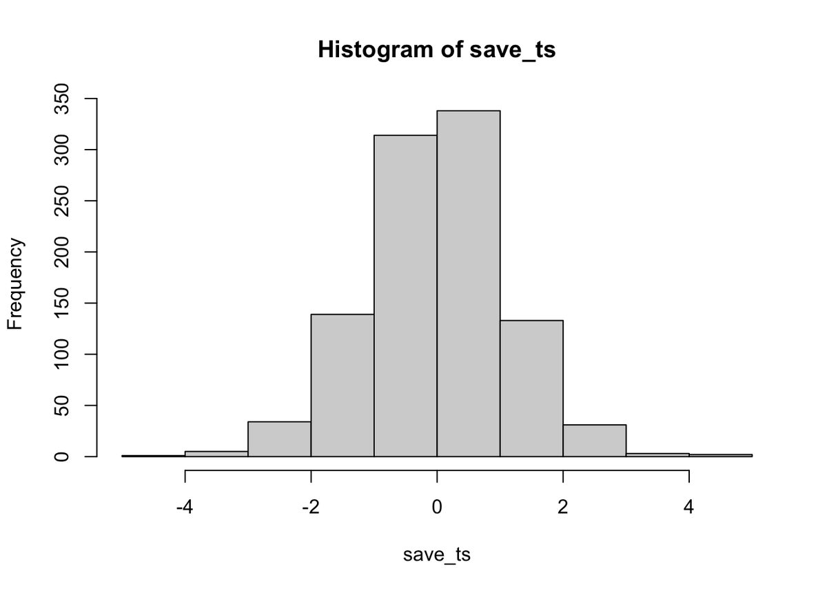
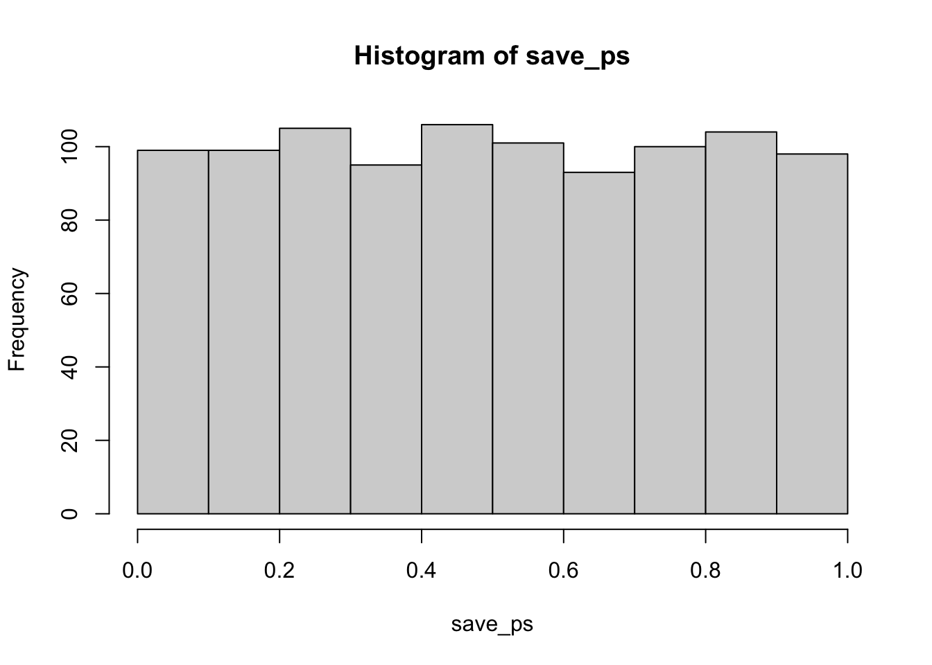
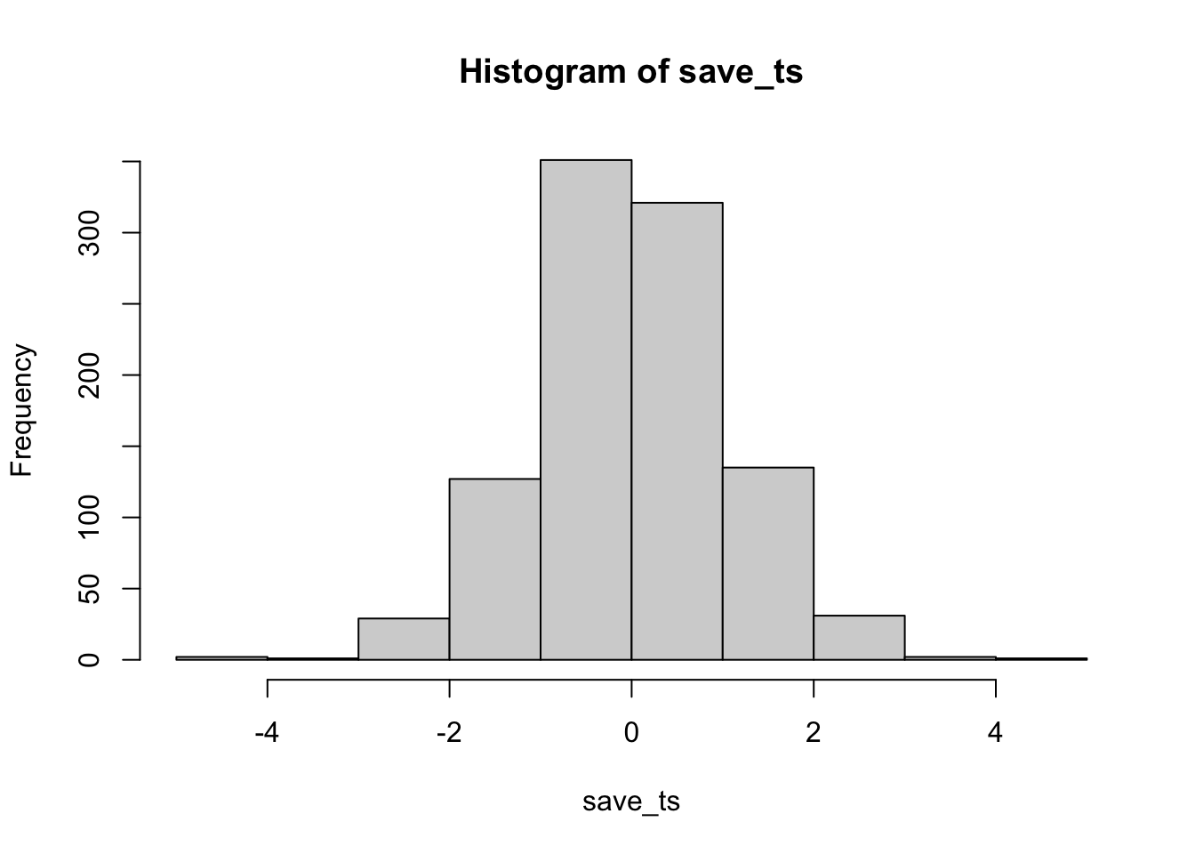
Histogram of 1,000 t-values simulated under the null hypothesis. They form a symmetric bell shape centered on zero, with nearly all values between -3 and 3 and the two tallest bars, over 300 simulations each, lying between -1 and 1. — Figure 6.15: 1000 simulated ts from the null distribution

Histogram of 1,000 p-values from t-tests simulated under the null. All ten bars sit near 100 simulations, an essentially uniform distribution showing that every p-value range between 0 and 1 is about equally likely by chance alone. — Figure 6.16: 1000 simulated ps from the null distribution

According to the simulation. When there are no differences between the conditions, and the samples are being pulled from the very same distribution, you get these two distributions for $t$ and $p$ . These again show how the null distribution of no differences behaves.

For any of these simulations, if you rejected the null-hypothesis (that your difference was only due to chance), you would be making a type I error. If you set your alpha criteria to $α equals.05$ , we can ask how many type I errors were made in these 1000 simulations. The answer is:

length(save_ps[save_ps<.05])
#> [1] 49
length(save_ps[save_ps<.05])/1000
#> [1] 0.049

We happened to make 49. The expectation over the long run is 5% type I error rates (if your alpha is.05).

What happens if there actually is a difference in the simulated data, let’s set one condition to have a larger mean than the other:

save_ps <- length(1000)
save_ts <- length(1000)
for ( i in 1:1000 ){
  condition_A <- rnorm(10,10,5)
  condition_B <- rnorm(10,13,5)
  differences <- condition_A - condition_B
  t_test <- t.test(differences, mu=0)
  save_ps[i] <- t_test$p.value
  save_ts[i] <- t_test$statistic
}

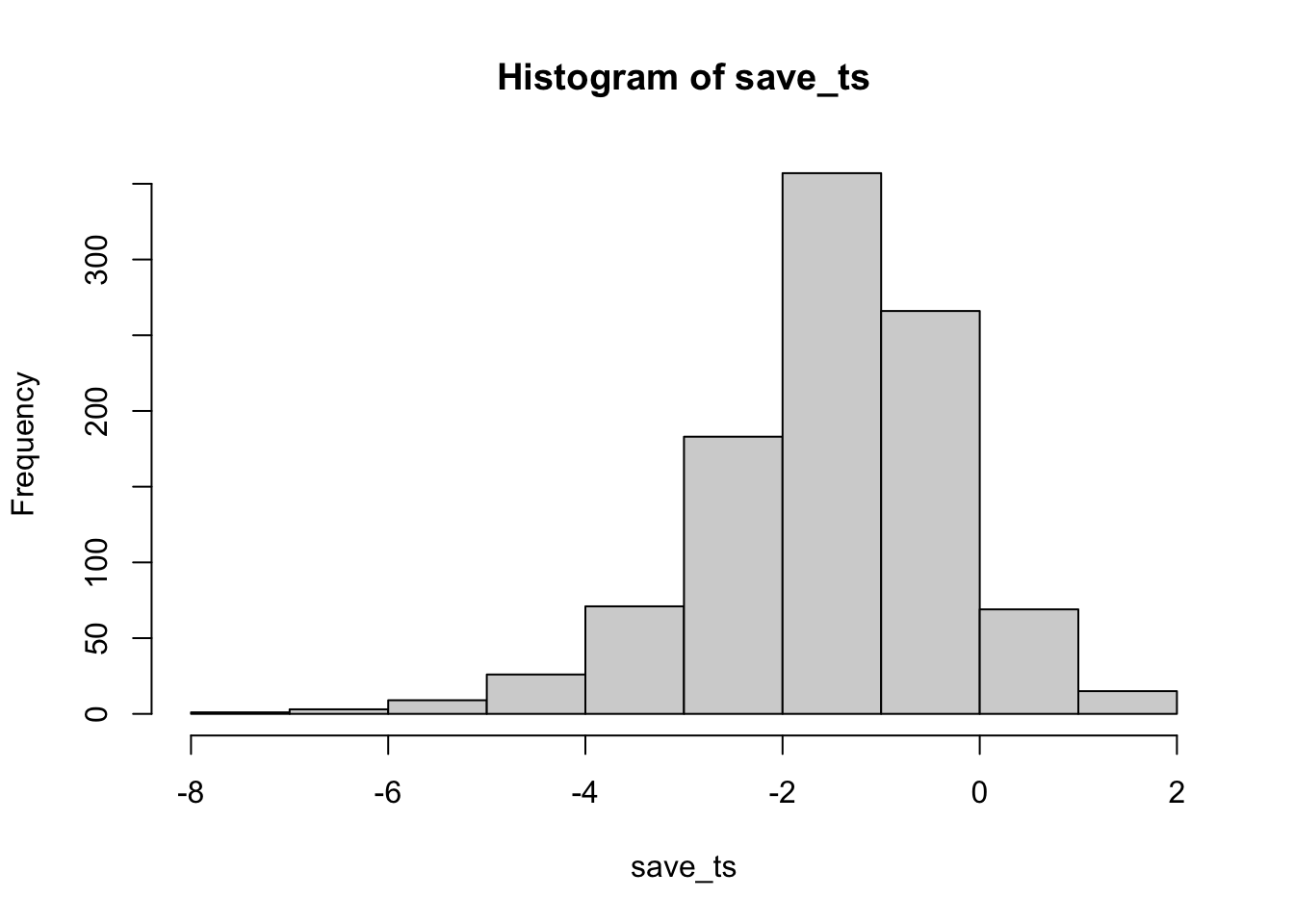
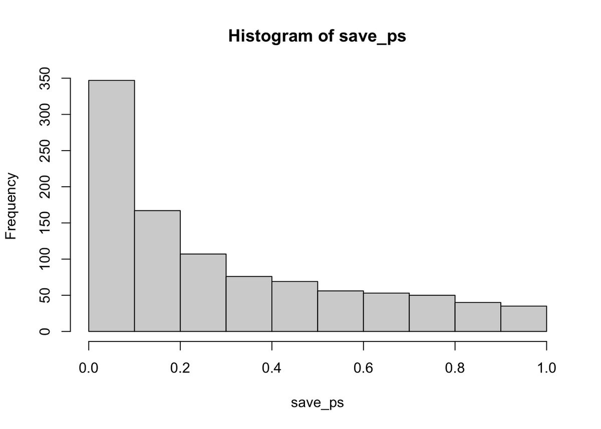
Histogram of 1,000 simulated t-values when a true difference exists. The bell shape is no longer centered on zero: it is shifted leftward, peaking between -2 and -1, with values ranging from about -8 up to 2. — Figure 6.17: 1000 ts when there is a true difference

Histogram of 1,000 simulated p-values when a true difference exists. The distribution is no longer flat: the leftmost bar, for p-values below 0.1, is tallest at about 350 simulations, and bar heights fall steadily toward 1, so small p-values now occur most often. — Figure 6.18: 1000 ps when there is a true difference

Now you can see that the $p$ -value distribution is skewed to the left. This is because when there is a true effect, you will get p-values that are less than.05 more often. Or, rather, you get larger $t$ values than you normally would if there were no differences.

In this case, we wouldn’t be making a type I error if we rejected the null when p was smaller than.05. How many times would we do that out of our 1000 experiments?

length(save_ps[save_ps<.05])
#> [1] 225
length(save_ps[save_ps<.05])/1000
#> [1] 0.225

We happened to get 225 simulations where p was less than.05, that’s only 0.225 experiments. If you were the researcher, would you want to run an experiment that would be successful only 0.225 of the time? I wouldn’t. I would run a better experiment.

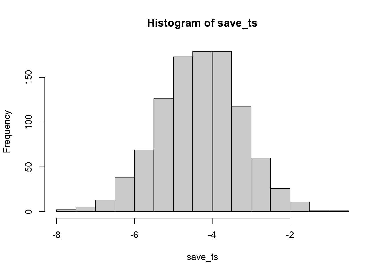
How would you run a better simulated experiment? Well, you could increase $n$ , the number of subjects in the experiment. Let’s increase $n$ from 10 to 100, and see what happens to the number of “significant” simulated experiments.

save_ps <- length(1000)
save_ts <- length(1000)
for ( i in 1:1000 ){
  condition_A <- rnorm(100,10,5)
  condition_B <- rnorm(100,13,5)
  differences <- condition_A - condition_B
  t_test <- t.test(differences, mu=0)
  save_ps[i] <- t_test$p.value
  save_ts[i] <- t_test$statistic
}

Histogram of 1,000 simulated t-values for samples of n=100 when a real effect exists. The bell-shaped distribution is centered near -4 and spans roughly -8 to -1, sitting almost entirely away from the zero that chance alone would produce. — Figure 6.19: 1000 ts for n =100, when there is a true effect

Show expected output

[1] 988
[1] 0.988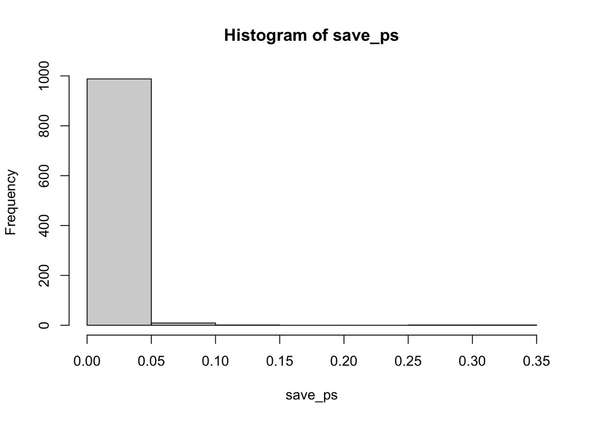

Histogram of 1,000 simulated p-values from experiments with n=100 and a real effect. Nearly all of the p-values pile into the single leftmost bar below 0.05, showing that with this sample size the test detects the true effect on almost every simulated run. — Figure 6.20: 1000 ps for n =100, when there is a true effect

Cool, now almost all of the experiments show a $p$ -value of less than.05 (using a two-tailed test, that’s the default in R). See, you could use this simulation process to determine how many subjects you need to reliably find your effect.

6.6.3 Simulating an independent samples t.test

Just change the t.test function like so… this is for the null, assuming no difference between groups.

save_ps <- length(1000)
save_ts <- length(1000)
for ( i in 1:1000 ){
  group_A <- rnorm(10,10,5)
  group_B <- rnorm(10,10,5)
  t_test <- t.test(group_A, group_B, paired=FALSE, var.equal=TRUE)
  save_ps[i] <- t_test$p.value
  save_ts[i] <- t_test$statistic
}

Histogram of 1,000 simulated t-values forming a symmetric bell shape centered on zero, with almost all values between -3 and 3 and the two tallest bars, over 300 simulations each, between -1 and 1. — Figure 6.21: 1000 ts for n =10 per group, when there is no difference between the groups

Show expected output

[1] 48
[1] 0.048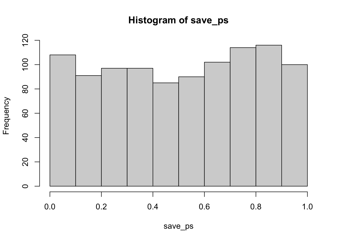

Histogram of 1,000 simulated p-values spread across the full 0-to-1 range. All ten bars are similar in height, roughly 85 to 116 simulations each, an approximately flat distribution with no pile-up of small p-values below 0.05. — Figure 6.22: 1000 ps for n =10 per group, when there is no difference between the groups

Adapted from Answering Questions with Data: Introductory Statistics for Psychology Students, by Matthew J. C. Crump (Brooklyn College of CUNY), crumplab.com/statistics, licensed under CC BY-SA 4.0. Portions adapt Danielle Navarro's Learning Statistics with R (CC BY-SA). Changes were made; this adaptation is distributed under the same license. License: CC-BY-SA-4.0.