
6.2 One-sample t-test: A new t-test
Now we are ready to talk about t-test. We will talk about three of them. We start with the one-sample t-test.
Commonly, the one-sample t-test is used to estimate the chances that your sample came from a particular population. Specifically, you might want to know whether the mean that you found from your sample, could have come from a particular population having a particular mean.
Straight away, the one-sample t-test becomes a little confusing (and I haven’t even described it yet). Officially, it uses known parameters from the population, like the mean of the population and the standard deviation of the population. However, most times you don’t know those parameters of the population! So, you have to estimate them from your sample. Remember from the chapters on descriptive statistics and sampling, our sample mean is an unbiased estimate of the population mean. And, our sample standard deviation (the one where we divide by n-1) is an unbiased estimate of the population standard deviation. When Gosset developed the t-test, he recognized that he could use these estimates from his samples, to make the t-test. Here is the formula for the one sample t-test, we first use words, and then become more specific:
6.2.1 Formulas for one-sample t-test
Where, s is the sample standard deviation.
Some of you may have gone cross-eyed looking at all of this. Remember, we’ve seen it before when we divided our mean by the standard deviation in the first bit. The t-test is just a measure of a sample mean, divided by the standard error of the sample mean. That is it.
6.2.2 What does t represent?
gives us a measure of confidence, just like our previous ratio for dividing the mean by a standard deviations. The only difference with , is that we divide by the standard error of mean (remember, this is also a standard deviation, it is the standard deviation of the sampling distribution of the mean)
is a property of the data that you collect. You compute it with a sample mean, and a sample standard error (there’s one more thing in the one-sample formula, the population mean, which we get to in a moment). This is why we call , a sample-statistic. It’s a statistic we compute from the sample.
What kinds of numbers should we expect to find for these ? How could we figure that out?
Let’s start small and work through some examples. Imagine your sample mean is 5. You want to know if it came from a population that also has a mean of 5. In this case, what would be? It would be zero: we first subtract the sample mean from the population mean, . Because the numerator is 0, will be zero. So, = 0, occurs, when there is no difference.
Let’s say you take another sample, do you think the mean will be 5 every time, probably not. Let’s say the mean is 6. So, what can be here? It will be a positive number, because 6-5= +1. But, will be +1? That depends on the standard error of the sample. If the standard error of the sample is 1, then could be 1, because 1/1 = 1.
If the sample standard error is smaller than 1, what happens to ? It gets bigger right? For example, 1 divided by 0.5 = 2. If the sample standard error was 0.5, would be 2. And, what could we do with this information? Well, it be like a measure of confidence. As gets bigger we could be more confident in the mean difference we are measuring.
Can be smaller than 1? Sure, it can. If the sample standard error is big, say like 2, then will be smaller than one (in our case), e.g., 1/2 = .5. The direction of the difference between the sample mean and population mean, can also make the become negative. What if our sample mean was 4. Well, then will be negative, because the mean difference in the numerator will be negative, and the number in the bottom (denominator) will always be positive (remember why, it’s the standard error, computed from the sample standard deviation, which is always positive because of the squaring that we did.).
So, that is some intuitions about what the kinds of values t can take. can be positive or negative, and big or small.
Let’s do one more thing to build our intuitions about what can look like. How about we sample some numbers and then measure the sample mean and the standard error of the mean, and then plot those two things against each each. This will show us how a sample mean typically varies with respect to the standard error of the mean.
In Figure 6.1, I pulled 1,000 samples of from a normal distribution (mean = 0, sd = 1). Each time I measured the mean and standard error of the sample. That gave two descriptive statistics for each sample, letting us plot each sample as dot in a scatter plot.
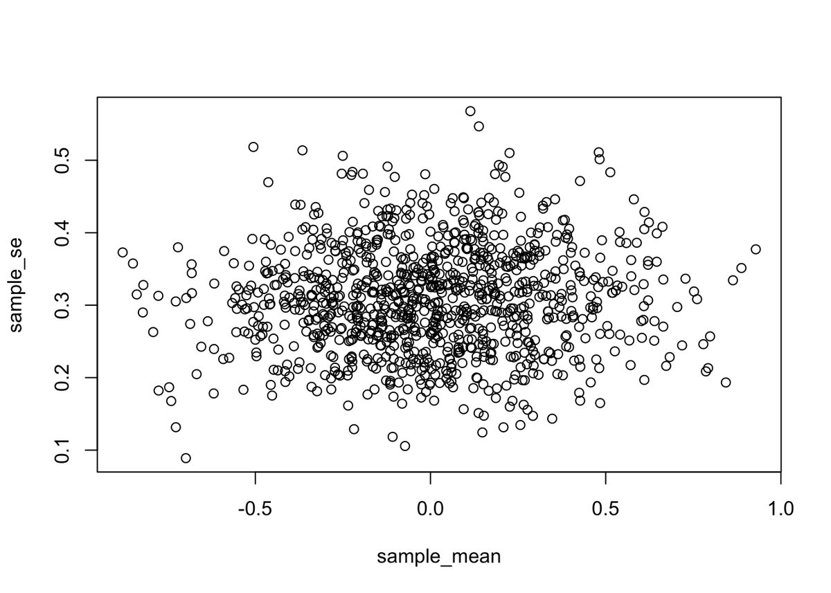
What we get is a cloud of dots. You might notice the cloud has a circular quality. There’s more dots in the middle, and fewer dots as they radiate out from the middle. The dot cloud shows us the general range of the sample mean, for example most of the dots are in between -1 and 1. Similarly, the range for the sample standard error is roughly between .2 and .5. Remember, each dot represents one sample.
We can look at the same data a different way. For example, rather than using a scatter plot, we can divide the mean for each dot by the standard error for each dot. Figure 6.2 shows the result in a histogram.
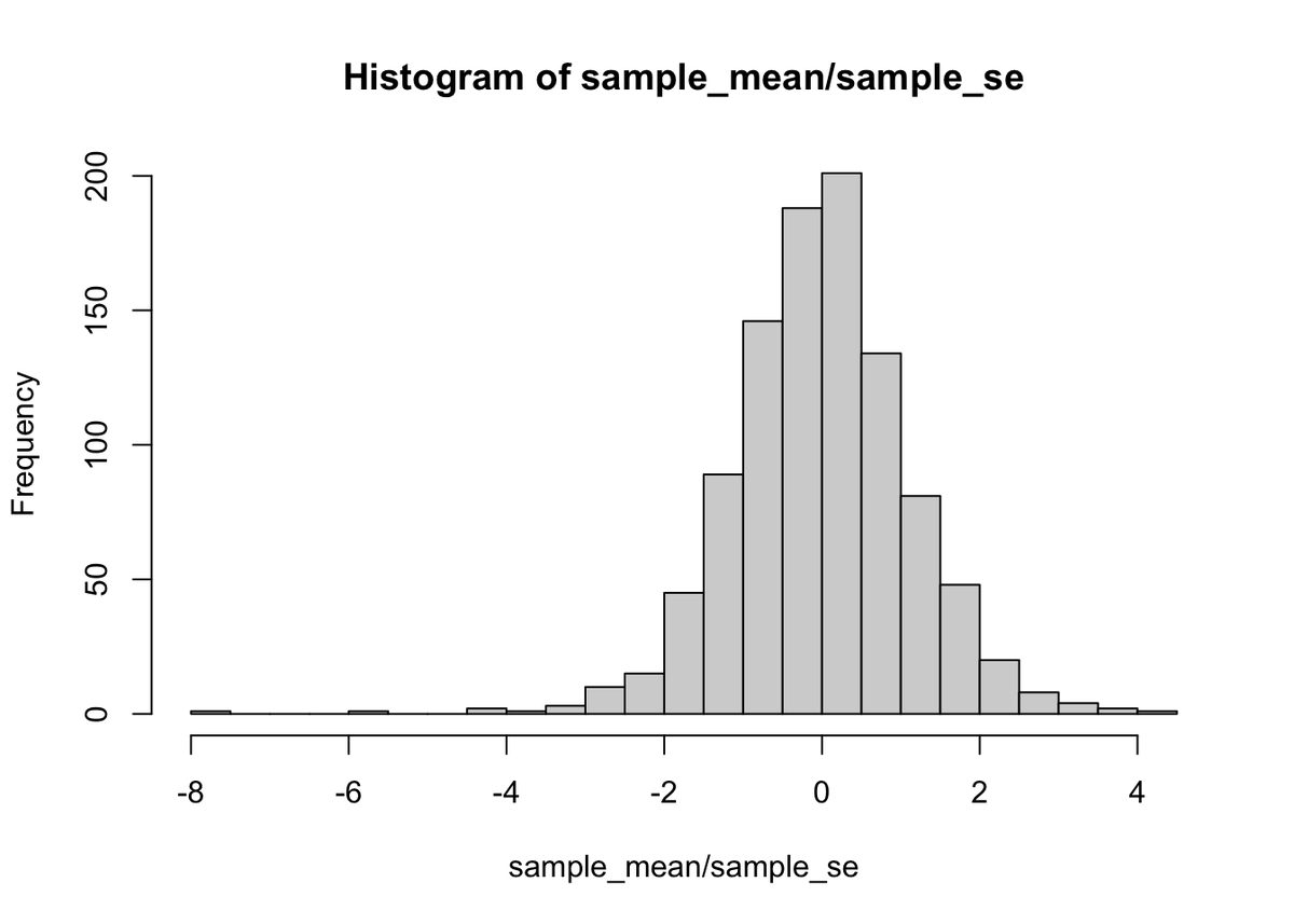
Interesting, we can see the histogram is shaped like a normal curve. It is centered on 0, which is the most common value. As values become more extreme, they become less common. If you remember, our formula for , was the mean divided by the standard error of the mean. That’s what we did here. This histogram is showing you a -distribution.
6.2.3 Calculating t from data
Let’s briefly calculate a t-value from a small sample. Let’s say we had 10 students do a true/false quiz with 10 questions on it. There’s a 50% chance of getting each answer correct.
Every student completes the 10 questions, we grade them, and then we find their performance (mean percent correct). What we want to know is whether the students were guessing. If they were all guessing, then the sample mean should be about 50%, it shouldn’t be different from chance, which is 50%. Let’s look at Table 6.1.
| students | scores | mean | Difference_from_Mean | Squared_Deviations |
|---|---|---|---|---|
| 1 | 50 | 61 | -11 | 121 |
| 2 | 70 | 61 | 9 | 81 |
| 3 | 60 | 61 | -1 | 1 |
| 4 | 40 | 61 | -21 | 441 |
| 5 | 80 | 61 | 19 | 361 |
| 6 | 30 | 61 | -31 | 961 |
| 7 | 90 | 61 | 29 | 841 |
| 8 | 60 | 61 | -1 | 1 |
| 9 | 70 | 61 | 9 | 81 |
| 10 | 60 | 61 | -1 | 1 |
| Sums | 610 | 610 | 0 | 2890 |
| Means | 61 | 61 | 0 | 289 |
| sd | 17.92 | |||
| SEM | 5.67 | |||
| t | 1.94003527336861 |
You can see the scores column has all of the test scores for each of the 10 students. We did the things we need to do to compute the standard deviation.
Remember the sample standard deviation is the square root of the sample variance, or:
The standard error of the mean, is the standard deviation divided by the square root of N
is the difference between our sample mean (61), and our population mean (50, assuming chance), divided by the standard error of the mean.
And, that is you how calculate , by hand. It’s a pain. I was annoyed doing it this way. In the lab, you learn how to calculate using software, so it will just spit out . For example in R, all you have to do is this:
scores <- c(50,70,60,40,80,30,90,60,70,60)
t.test(scores, mu=50)
Show expected output
 One Sample t-test

data:  scores
t = 1.9412, df = 9, p-value = 0.08415
alternative hypothesis: true mean is not equal to 50
95 percent confidence interval:
 48.18111 73.81889
sample estimates:
mean of x
       61
6.2.4 How does t behave?
If is just a number that we can compute from our sample (it is), what can we do with it? How can we use for statistical inference?
Remember back to the chapter on sampling and distributions, that’s where we discussed the sampling distribution of the sample mean. Remember, we made a lot of samples, then computed the mean for each sample, then we plotted a histogram of the sample means. Later, in that same section, we mentioned that we could generate sampling distributions for any statistic. For each sample, we could compute the mean, the standard deviation, the standard error, and now even , if we wanted to. We could generate 10,000 samples, and draw four histograms, one for each sampling distribution for each statistic.
This is exactly what I did, and the results are shown in the four panels of Figure 6.3 below. I used a sample size of 20, and drew random observations for each sample from a normal distribution, with mean = 0, and standard deviation = 1. Let’s look at the sampling distributions for each of the statistics. was computed assuming with the population mean assumed to be 0.
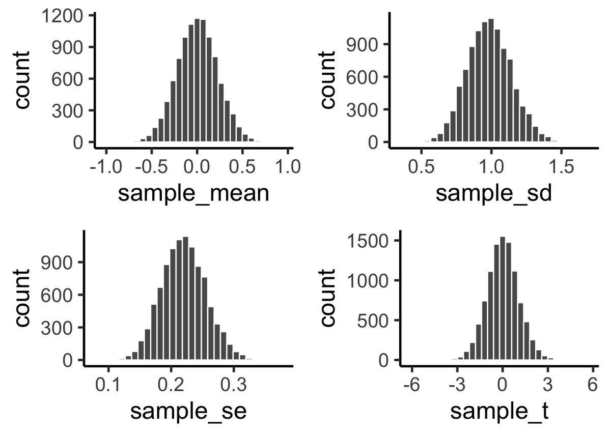
We see four sampling distributions. This is how statistical summaries of these summaries behave. We have used the word chance windows before. These are four chance windows, measuring different aspects of the sample. In this case, all of the samples came from the same normal distribution. Because of sampling error, each sample is not identical. The means are not identical, the standard deviations are not identical, sample standard error of the means are not identical, and the s of the samples are not identical. They all have some variation, as shown by the histograms. This is how samples of size 20 behave.
We can see straight away, that in this case, we are unlikely to get a sample mean of 2. That’s way outside the window. The range for the sampling distribution of the mean is around -.5 to +.5, and is centered on 0 (the population mean, would you believe!).
We are likely to get sample standard deviations of between .6 and 1.5, that is a different range, specific to the sample standard deviation.
Same thing with the sample standard error of the mean, the range here is even smaller, mostly between .1, and .3. You would rarely find a sample with a standard error of the mean greater than .3. Virtually never would you find one of say 1 (for this situation).
Now, look at . It’s range is basically between -3 and +3 here. 3s barely happen at all. You pretty much never see a 5 or -5 in this situation.
All of these sampling windows are chance windows, and they can all be used in the same way as we have used similar sampling distributions before (e.g., Crump Test, and Randomization Test) for statistical inference. For all of them we would follow the same process:
- Generate these distributions
- Look at your sample statistics for the data you have (mean, SD, SEM, and )
- Find the likelihood of obtaining that value or greater
- Obtain that probability
- See if you think your sample statistics were probable or improbable.
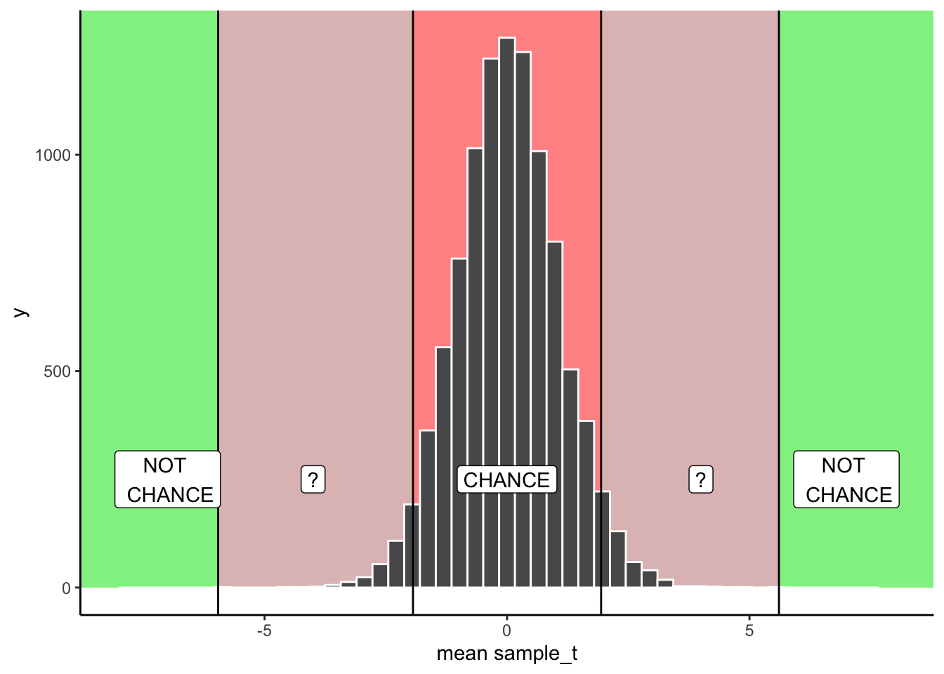
We’ll formalize this in a second. I just want you to know that what you will be doing is something that you have already done before. For example, in the Crump test and the Randomization test we focused on the distribution of mean differences. We could do that again here, but instead, we will focus on the distribution of values. We then apply the same kinds of decision rules to the distribution, as we did for the other distributions. Below you will see a graph you have already seen, except this time it is a distribution of s, not mean differences:
Remember, if we obtained a single from one sample we collected, we could consult the chance window in Figure 6.4 below to find out whether the we obtained from the sample was likely or unlikely to occur by chance.
6.2.5 Making a decision
From our early example involving the TRUE/FALSE quizzes, we are now ready to make some kind of decision about what happened there. We found a mean difference of 11. We found a = 1.9411765. The probability of this or larger occurring is = 0.0841503. We were testing the idea that our sample mean of 61 could have come from a normal distribution with mean = 50. The test tells us that the for our sample, or a larger one, would happen with p = 0.0841503. In other words, chance can do it a kind of small amount of time, but not often. In English, this means that all of the students could have been guessing, but it wasn’t that likely that were just guessing.
The next -test is called a paired samples t-test. And, spoiler alert, we will find out that a paired samples t-test is actually a one-sample t-test in disguise (WHAT!), yes it is. If the one-sample -test didn’t make sense to you, read the next section.
Adapted from Answering Questions with Data: Introductory Statistics for Psychology Students, by Matthew J. C. Crump (Brooklyn College of CUNY), crumplab.com/statistics, licensed under CC BY-SA 4.0. Portions adapt Danielle Navarro's Learning Statistics with R (CC BY-SA). Changes were made; this adaptation is distributed under the same license. License: CC-BY-SA-4.0.