
5.5 Calculating Electric Fields of Charge Distributions
The charge distributions we have seen so far have been discrete: made up of individual point particles. This is in contrast with a continuous charge distribution, which has at least one nonzero dimension. If a charge distribution is continuous rather than discrete, we can generalize the definition of the electric field. We simply divide the charge into infinitesimal pieces and treat each piece as a point charge.
Note that because charge is quantized, there is no such thing as a “truly” continuous charge distribution. However, in most practical cases, the total charge creating the field involves such a huge number of discrete charges that we can safely ignore the discrete nature of the charge and consider it to be continuous. This is exactly the kind of approximation we make when we deal with a bucket of water as a continuous fluid, rather than a collection of molecules.
Our first step is to define a charge density for a charge distribution along a line, across a surface, or within a volume, as shown in Figure 5.22.
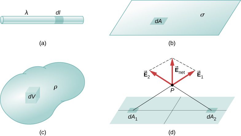
Definitions of charge density:
- charge per unit length (linear charge density); units are coulombs per meter (C/m)
- charge per unit area (surface charge density); units are coulombs per square meter
- charge per unit volume (volume charge density); units are coulombs per cubic meter
Then, for a line charge, a surface charge, and a volume charge, the summation in Equation 5.4 becomes an integral and is replaced by , , or , respectively:
The integrals are generalizations of the expression for the field of a point charge. They implicitly include and assume the principle of superposition. The “trick” to using them is almost always in coming up with correct expressions for dl, dA, or dV, as the case may be, expressed in terms of r, and also expressing the charge density function appropriately. It may be constant; it might be dependent on location.
Note carefully the meaning of r in these equations: It is the distance from the charge element to the location of interest, (the point in space where you want to determine the field). However, don’t confuse this with the meaning of ; we are using it and the vector notation to write three integrals at once. That is, Equation 5.9 is actually
In the case of a finite line of charge, note that for , dominates the L in the denominator, so that Equation 5.12 simplifies to
If you recall that , the total charge on the wire, we have retrieved the expression for the field of a point charge, as expected.
In the limit , on the other hand, we get the field of an infinite straight wire, which is a straight wire whose length is much, much greater than either of its other dimensions, and also much, much greater than the distance at which the field is to be calculated:
An interesting artifact of this infinite limit is that we have lost the usual dependence that we are used to. This will become even more intriguing in the case of an infinite plane.
As , Equation 5.14 reduces to the field of an infinite plane, which is a flat sheet whose area is much, much greater than its thickness, and also much, much greater than the distance at which the field is to be calculated:
Note that this field is constant. This surprising result is, again, an artifact of our limit, although one that we will make use of repeatedly in the future. To understand why this happens, imagine being placed above an infinite plane of constant charge. Does the plane look any different if you vary your altitude? No—you still see the plane going off to infinity, no matter how far you are from it. It is important to note that Equation 5.15 is because we are above the plane. If we were below, the field would point in the direction.
Summary
- A very large number of charges can be treated as a continuous charge distribution, where the calculation of the field requires integration. Common cases are:
- one-dimensional (like a wire); uses a line charge density
- two-dimensional (metal plate); uses surface charge density
- three-dimensional (metal sphere); uses volume charge density
- The “source charge” is a differential amount of charge dq. Calculating dq depends on the type of source charge distribution:
- Symmetry of the charge distribution is usually key.
- Important special cases are the field of an “infinite” wire and the field of an “infinite” plane.
Conceptual Questions
Give a plausible argument as to why the electric field outside an infinite charged sheet is constant.
At infinity, we would expect the field to go to zero, but because the sheet is infinite in extent, this is not the case. Everywhere you are, you see an infinite plane in all directions.
Compare the electric fields of an infinite sheet of charge, an infinite, charged conducting plate, and infinite, oppositely charged parallel plates.
Describe the electric fields of an infinite charged plate and of two infinite, charged parallel plates in terms of the electric field of an infinite sheet of charge.
The infinite charged plate would have everywhere. The field would point toward the plate if it were negatively charged and point away from the plate if it were positively charged. The electric field of the parallel plates would be zero between them if they had the same charge, and E would be everywhere else. If the charges were opposite, the situation is reversed, zero outside the plates and between them.
A negative charge is placed at the center of a ring of uniform positive charge. What is the motion (if any) of the charge? What if the charge were placed at a point on the axis of the ring other than the center?
Problems
A thin conducting plate 1.0 m on the side is given a charge of . An electron is placed 1.0 cm above the center of the plate. What is the acceleration of the electron?
Calculate the magnitude and direction of the electric field 2.0 m from a long wire that is charged uniformly at
Two thin conducting plates, each 25.0 cm on a side, are situated parallel to one another and 5.0 mm apart. If electrons are moved from one plate to the other, what is the electric field between the plates?
The charge per unit length on the thin rod shown below is . What is the electric field at the point P? (Hint: Solve this problem by first considering the electric field at P due to a small segment dx of the rod, which contains charge . Then find the net field by integrating over the length of the rod.)

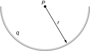
The charge per unit length on the thin semicircular wire shown below is . What is the electric field at the point P?
Two thin parallel conducting plates are placed 2.0 cm apart. Each plate is 2.0 cm on a side; one plate carries a net charge of and the other plate carries a net charge of What is the charge density on the inside surface of each plate? What is the electric field between the plates?
A thin conducting plate 2.0 m on a side is given a total charge of . (a) What is the electric field above the plate? (b) What is the force on an electron at this point? (c) Repeat these calculations for a point 2.0 cm above the plate. (d) When the electron moves from 1.0 to 2,0 cm above the plate, how much work is done on it by the electric field?
A total charge q is distributed uniformly along a thin, straight rod of length L (see below). What is the electric field at
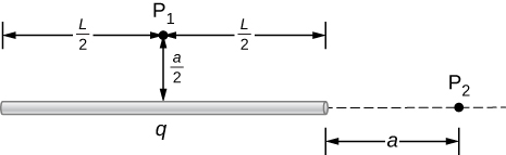
At :
At Put the origin at the end of L.
Charge is distributed along the entire x-axis with uniform density How much work does the electric field of this charge distribution do on an electron that moves along the y-axis from
Charge is distributed along the entire x-axis with uniform density and along the entire y-axis with uniform density Calculate the resulting electric field at (a) and (b)
a. ; b.
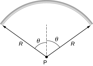
A rod bent into the arc of a circle subtends an angle at the center P of the circle (see below). If the rod is charged uniformly with a total charge Q, what is the electric field at P?
A proton moves in the electric field (a) What are the force on and the acceleration of the proton? (b) Do the same calculation for an electron moving in this field.
a. ,
;
b. ,
An electron and a proton, each starting from rest, are accelerated by the same uniform electric field of 200 N/C. Determine the distance and time for each particle to acquire a kinetic energy of
A spherical water droplet of radius carries an excess 250 electrons. What vertical electric field is needed to balance the gravitational force on the droplet at the surface of the earth?
,
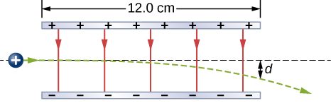
A proton enters the uniform electric field produced by the two charged plates shown below. The magnitude of the electric field is and the speed of the proton when it enters is What distance d has the proton been deflected downward when it leaves the plates?
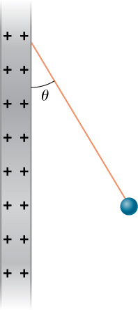
Shown below is a small sphere of mass 0.25 g that carries a charge of The sphere is attached to one end of a very thin silk string 5.0 cm long. The other end of the string is attached to a large vertical conducting plate that has a charge density of What is the angle that the string makes with the vertical?
,
,
,
This is independent of the length of the string.
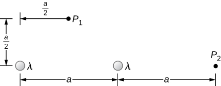
Two infinite rods, each carrying a uniform charge density are parallel to one another and perpendicular to the plane of the page. (See below.) What is the electrical field at
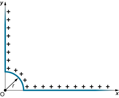
Positive charge is distributed with a uniform density along the positive x-axis from along the positive y-axis from and along a arc of a circle of radius r, as shown below. What is the electric field at O?
circular arc ,
,
,
;
y-axis: ;
x-axis: ,
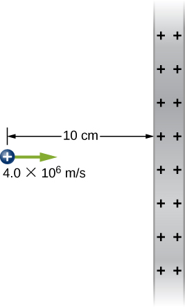
From a distance of 10 cm, a proton is projected with a speed of directly at a large, positively charged plate whose charge density is (See below.) (a) Does the proton reach the plate? (b) If not, how far from the plate does it turn around?
A particle of mass m and charge moves along a straight line away from a fixed particle of charge Q. When the distance between the two particles is is moving with a speed (a) Use the work-energy theorem to calculate the maximum separation of the charges. (b) What do you have to assume about to make this calculation? (c) What is the minimum value of such that escapes from Q?
a. , ; b. is negative; therefore, ,