11.1 Hypothesis Testing for Mean μ (z-test)

Watch demo video

Suppose a random sample of size $n$ is drawn from a population with unknow mean $\mu$ and either the standard deviation $\sigma$ is given or the sample size is large.

To test a hypothesis about the mean $\mu$ of the form:

$H_0:\mu =\mu_0$

$H_a:\mu < \mu_0$ smaller

OR:

$H_0:\mu =\mu_0$

$H_a:\mu > \mu_0$ greater

OR:

$H_0:\mu =\mu_0$

$H_a:\mu \ne \mu_0$ two-sided

we use the following test-statistic

$z=\frac{\bar x - \mu_o}{\frac{\sigma}{\sqrt{n}}}$

Use the function z_test_mean below with arguments: null_mean = $\mu_o$ , sigma = $\sigma$ , sample_mean = $\bar{x}$ , n, alternative = 'smaller' OR 'greater' OR 'two-sided'. By default it is set to 'two-sided'.

# z test with alternative 'smaller' or 'greater' or 'two-sided'
def z_test_mean(null_mean,sigma,sample_mean,n,alternative='two-sided'):  
    from scipy import stats
    z = (sample_mean-null_mean)/(sigma/n**.5)
    if alternative == 'smaller':
        pv = stats.norm.cdf(z,0,1)
    elif alternative == 'greater':
        pv = 1-stats.norm.cdf(z,0,1)
    elif alternative == 'two-sided':
        if z< 0: 
            pv = 2*stats.norm.cdf(z,0,1)
        else: pv = 2*(1-stats.norm.cdf(z,0,1))
    else:
        print("alternative option error")
    return print("z test statistic = ", z, "and p-value = ",pv)

Example: The president of a company claims that the average number of minutes employees waste time surfing the internet is more than 100 minutes a day. The population number of hours wasted is normally distributed with standard deviation of 10 minutes. A random sample of 19 employees from this company has a mean of 105 minutes. Do this sample data provide evidence that the mean wasted time for this company is more than 100 minutes? Use $\alpha = 0.05$ .

$H_o:\mu = 100$

$H_a: \mu > 100$

Use the z_test_mean function above with arguments: null_mean = 100, sigma = 10, sample_mean = 105, n = 19, alternative = 'greater' (more than 100).

Click play button on code above def z_test_mean
Click + Code
Type z_test_mean(100,10,105,19,'greater')
Click play button

z_test_mean(100,10,105,19,'greater')

Show expected output

z test statistic =  2.179449471770337 and p-value =  0.014649147202275281

Interpretation: p-value = 0.014649 < $\alpha$ = 0.05. The null hypothesis is rejected.

Alternatively, compare z = (sample_mean-null_mean)/(sigma/n**.5) with the critical z stats.norm.ppf(1-.05,0,1) = 1.6448 see code below. $z=2.179449471770337>1.6448536269514722$ thus reject the null-hypothesis.

A dark blue standard normal curve, drawn at ten times the usual density so its peak reads about 4 rather than 0.4. Its right-hand tail is shaded red from the critical value z* = 1.645 outward — the rejection region for a test at the 5% level. A fixed green vertical line stands at the observed z of 2.18, which at these settings falls inside the shaded region, so the null hypothesis is rejected. Moving the critical value carries the edge of the shading past the observed value and reverses that decision with none of the data changing. Adjustable parameter: Critical value z* (c) = 1.64. Viewing window: x from -4 to 4, y from -0.77 to 4.17. — The blue curve is the standard normal (drawn at ten times the density, so its peak reads 3.99 rather than 0.399); the shaded tail is the rejection region, and its left edge z* is the slider. The green line is this example's observed z = 2.179449471770337 and never moves. Start at the section's z* = 1.6449 - alpha = 0.05 - and the observed value is inside the shaded region, so the null is rejected. Drag z* right to 2.3263 (alpha = 0.01) and the green line falls OUTSIDE the region: the same data, the same test, the opposite decision, because alpha changed. Drag it to 2.179449 and the boundary lands exactly on the observed value - that is what a p-value is, the alpha at which the decision flips, and here it is 0.014649. A printed picture of one shaded tail can state that definition; only a draggable one lets you watch the decision change.

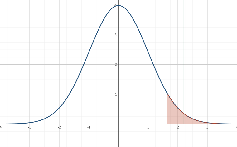
from scipy import stats
stats.norm.ppf(1-0.05,0,1)   # right-tailed test

Show expected output

1.6448536269514722

Example: A government official claims that the average recovery time for Covid19 patients with severe symptoms is 6 weeks. A random sample of 23 patients with severe symptoms has a mean recovery time of 5.4 weeks with standard deviation of 1.1 weeks. Assume recovery time is normally distributed with standard deviation of 1.5 ( $\sigma$ ) weeks. Test the government's official claim at $\alpha$ of 0.05. Use the z_test_mean function below.

# z test with alternative 'smaller' or 'greater' or 'two-sided'
def z_test_mean(null_mean,sigma,sample_mean,n,alternative='two-sided'):  
    from scipy import stats
    z = (sample_mean-null_mean)/(sigma/n**.5)
    if alternative == 'smaller':
        pv = stats.norm.cdf(z,0,1)
    elif alternative == 'greater':
        pv = 1-stats.norm.cdf(z,0,1)
    elif alternative == 'two-sided':
        if z< 0: 
            pv = 2*stats.norm.cdf(z,0,1)
        else: pv = 2*(1-stats.norm.cdf(z,0,1))
    else:
        print("alternative option error")
    return print("z test statistic = ", z, "and p-value = ",pv)

null_mean=6,sigma=1.5,sample_mean=5.4,n=23,alternative='two-sided

z_test_mean(6,1.5,5.4,23,'two-sided')

Show expected output

z test statistic =  -1.9183326093250865 and p-value =  0.05506885012079212

Interpretation: Because the p-value 0.05506885012079212 is not less than 0.05, fail to reject the null hypothesis. There is no sufficient evidence to reject the official's claim.

Example: The work week of a particular organization workers is normally distributed with a mean of 47 hours. A newly hired manager at this company believes that employees average work hours is different from 47. She randomly asks 12 workers for the lengths in hours of their work week. Their responses are shown below. Test the claim using a 10% level of significance. The population standard deviation is 5.

Hours: 46, 43, 55, 50, 46, 67, 48, 47, 48, 49, 55, 54

$H_o:\mu = 47$

$H_a: \mu \ne 47$

We need to find the mean and sample size of the data before we call the function, z_test_mean.

import numpy as np
x = [46, 43, 55, 50, 46, 67, 48, 47, 48, 49, 55, 54]

m = np.mean(x)
n = np.size(x)
print('mean is',m,'\n n is',n)

Show expected output

mean is 50.666666666666664 
 n is 12

Using the sample_mean=m and n from the above code, we call z_test_mean with arguments:47,5,50.666667,12,'two-sided'. But by default the function is set to 'two-sided'

Try it in XYZ Crunch

The 12 work weeks, tested from their mean

np.mean has already turned the twelve responses into one number, and from there the test needs nothing else about the data. The link carries mu0 = 47, x-bar = 50.6666667, sigma = 5, n = 12, Two-tailed, alpha = 0.1 and reports Z-statistic 2.540341, P-value 0.011074 and Reject H0 - the cell's own output and the interpretation's verdict. The x-bar in the link is the rounded 50.6666667 the call below passes, not the full 50.666666666666664; the difference first shows up in the seventh decimal of z, which is a fair demonstration of how little rounding a mean costs you here.

Z-Test, mu0 = 47, x-bar = 50.6666667, sigma = 5, n = 12, two-tailed at alpha = 0.1: z = 2.540341, p = 0.011074, Reject H0

z_test_mean(47,5,50.6666667,12)   #you need to run the ttestmean function above first before you call it.

Show expected output

z test statistic =  2.540341207528364 and p-value =  0.011074436944822352

Interpretation: The p-value 0.011074436944822352 is less than $\alpha = 0.10$ . Reject the null hypothesis.

Adapted from Python for Introductory Statistics, by Simon Aman (Truman College, City Colleges of Chicago), licensed under CC BY 4.0. Changes were made: reformatted as an accessible XYZ web edition with live in-browser code cells. License: CC-BY-4.0.