
8.2 Binomial Probability
If an experiment consists of identical and independent trials, with probability of success (remains the same for each trial), then the random variable defined as the number of successes in trials is a binomial random variable and the probability of successes is given by:
where
The syntax for , given n and p is
from scipy import stats
stats.binom.pmf(x,n,p)
The syntax for cumulative probability , given n and p is
from scipy import stats
stats.binom.cdf(x,n,p)
The syntax for mean and standard deviation is given by:
from scipy import stats
stats.binom.mean(n,p)
stats.binom.std(n,p)
Example: Find if
Here x=10, n=12 and p=0.6.
from scipy import stats
stats.binom.pmf(10, 12, 0.6)
Show expected output
0.06385228185599987Example: For a Binomial distribution with 12 number of trials and probability of success 0.6, find the cumulative probabilities . Here x=2, p=0.6 and n=12.
from scipy import stats
stats.binom.cdf(k=2, n=12, p=0.6)  # same as stats.binom.cdf(2, 12, 0.6)
Show expected output
0.00281018368Interpretation:
Example: A manufacturing machine has a 5% defect rate. Write a scipy.stats program to compute the following:
- If 6 items are chosen at random, what is the probability of exactly 2 defects.
from scipy import stats

stats.binom.pmf(2,6,0.05)
Show expected output
0.030543984375000013Interpretation: The probability of exactly two out of six defects is 0.030543984375000013
Example: A manufacturing machine has a 5% defect rate. Write a scipy.stats program to compute the following:
- If 6 items are chosen at random, what is the probability that 3 or less will have a defect?
from scipy import stats
stats.binom.cdf(3,6,0.05)
Show expected output
0.99991359375Interpretation: The probability of 3 or less defects is 0.99991359375
Example: A manufacturing machine has a 5% defect rate. Write a scipy.stats program to compute the following:
- If 6 items are chosen at random, what is the probability that at least two defects?
from scipy import stats
1-stats.binom.cdf(1,6,0.05)
Show expected output
0.03277382812500007Interpretation: The probability of at least two defects is 0.03277382812500007
Example: 20% of cars fail emission inspections in IL. If 15 cars are randomly selected, what is the probability that exactly three fail.
Here x=3, p=.2 and n=15
from scipy import stats
stats.binom.pmf(3,15,.2)
Show expected output
0.2501388953190411Interpretation:
Example: 20% of cars fail emission inspections in IL. If 15 cars are randomly selected, what is the probability that at most five fail?
Here x=5, p=.2 and n=15 (Cumulative)
from scipy import stats
stats.binom.cdf(5,15,.2)
Show expected output
0.938948570382336Interpretation:
Example: 20% of cars fail emission inspections in IL. If 15 cars are randomly selected, what is the probability that at least five fail?
from scipy import stats
1 - stats.binom.cdf(4,15,.2)
Show expected output
0.16423372393676794Interpretation:
Example: 20% of cars fail emission inspections in IL. 15 cars are randomly selected from IL. Make a probability distribution table for each outcome.
from scipy import stats
import numpy as np
x = np.arange(0,15+1)  #generates [0,1,2,..,15]
y = stats.binom.pmf(x,15,.2)

prob = zip(x,y)
list(prob)
Show expected output
[(0, 0.035184372088831996),
 (1, 0.13194139533312002),
 (2, 0.23089744183296135),
 (3, 0.2501388953190411),
 (4, 0.18760417148928044),
 (5, 0.10318229431910414),
 (6, 0.04299262263296016),
 (7, 0.013819057274880048),
 (8, 0.0034547643187200112),
 (9, 0.000671759728640003),
 (10, 0.00010076395929600008),
 (11, 1.1450449920000038e-05),
 (12, 9.542041600000053e-07),
 (13, 5.505024000000039e-08),
 (14, 1.9660800000000028e-09),
 (15, 3.276800000000002e-11)]
Interpretation:
| x | probability |
|---|---|
| 0 | 0.035184372088831996 |
| 1 | 0.13194139533312002 |
| 2 | 0.23089744183296135 |
| 3 | 0.2501388953190411 |
| 4 | 0.18760417148928044 |
| 5 | 0.10318229431910414 |
| 6 | 0.04299262263296016 |
| 7 | 0.013819057274880048 |
| 8 | 0.0034547643187200112 |
| 9 | 0.000671759728640003 |
| 10 | 0.00010076395929600008 |
| 11 | 1.1450449920000038e-05 |
| 12 | 9.542041600000053e-07 |
| 13 | 5.505024000000039e-08 |
| 14 | 1.9660800000000028e-09 |
| 15 | 3.276800000000002e-11 |
Binomial Plot
Use the function binomplot below to plot a binomial distribution with probability p and number of trials n.
# binomial graph with n and p
def binomplot(n,p):
  from scipy import stats
  import numpy as np
  import matplotlib.pyplot as plt

  x = np.arange(0,n+1)
  y = stats.binom.pmf(x,n,p)
  plt.bar(x,y,width=0.2)

  plt.suptitle("Binomial Plot")
  plt.xlabel("x values")
  plt.ylabel("probability")

  return plt.show()
Example: plot a binomial distribution with n=10 and p=0.6
binomplot(10,.6) # run the binomplot function above first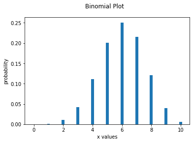
Example: Graph a Binomial Probability Distribution with n=10 and p=.3.
binomplot(10,.3) # run the binomplot function above first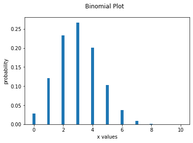
Adapted from Python for Introductory Statistics, by Simon Aman (Truman College, City Colleges of Chicago), licensed under CC BY 4.0. Changes were made: reformatted as an accessible XYZ web edition with live in-browser code cells. License: CC-BY-4.0.