4.1 Statistical Inference and Confidence Intervals

Learning Outcomes

By the end of this section, you should be able to:

Estimate parameters, create confidence intervals, and calculate sample size requirements.
Apply bootstrapping methods for parameter estimation.
Use Python to calculate confidence intervals and conduct hypothesis tests.

Data scientists interested in inferring the value of a population truth or parameter such as a population mean or a population proportion turn to inferential statistics. A data scientist is often interested in making generalizations about a population based on the characteristics derived from a sample; inferential statistics allows a data scientist to draw conclusions about a population based on sample data. In addition, inferential statistics is used by data scientists to assess model performance and compare different algorithms in machine learning application. Inferential statistics provides methods for generating predictive forecasting models, and this allows data scientists to generate predictions and trends to assist in effective and accurate decision-making. In this section, we explore the use of confidence intervals, which is used extensively in inferential statistical analysis.

We begin by introducing confidence intervals, which are used to estimate the range within which a population parameter is likely to fall. We discuss estimation of parameters for the mean both when the standard deviation is known and when it is not known. We discuss sample size determination, building on the sampling techniques presented in Collecting and Preparing Data. And we discuss bootstrapping, a method used to construct a confidence interval based on repeated sampling. Hypothesis Testing will move on to hypothesis testing, which is used to make inferences about unknown parameters.

Estimating Parameters with Confidence Intervals

A point estimate is a single value that is used to estimate a population parameter. For example, a sample mean is a point estimate that is representative of the true population mean in that the sample mean is used as an estimate for the unknown population mean. When researchers collect data from a sample to make inferences about a population, they calculate a point estimate based on the observed sample data. (See Survey Design and Implementation for coverage of sampling techniques.) The point estimate serves as the best guess or approximation for the parameter's actual value.

A confidence interval estimates the range within which a population parameter, such as a mean or a proportion, is likely to fall. The confidence interval provides a level of uncertainty associated with the estimate and is expressed as a range of values. A confidence interval will provide both a lower and an upper bound for the population parameter, where the point estimate is centered within the interval.

Table 4.1 describes the point estimates and corresponding population parameters for the mean and proportion.

**Table 4.1**
	Population Parameter	Point Estimate
Mean	Population mean is denoted as $µ$ .	Point estimate is the sample mean $\bar{x}$ .
Proportion	Population proportion is denoted as $p$ .	Point estimate is the sample proportion $p ^$ .

Let’s say a researcher is interested in estimating the mean income for all residents of California. Since it is not feasible to collect data from every resident of California, the researcher selects a random sample of 1,000 residents and calculates the sample mean income for these 1,000 people. This average income estimate from the sample then provides an estimate for the population mean income of all California residents. The sample mean is chosen as the point estimate for the population mean in that the sample mean provides the most unbiased estimate for the population mean. In the same way, the sample proportion provides the most unbiased estimate for the population proportion. An unbiased estimator is a statistic that provides an accurate estimate for the corresponding population parameter without overestimating or underestimating the parameter.

In order to calculate a confidence interval, two quantities are needed:

The point estimate
The margin of error

As noted, the point estimate is a single number that is used to estimate the population parameter. The margin of error (usually denoted by E) provides an indication of the maximum error of the estimate. The margin of error can be viewed as the maximum distance around the point estimate where the population parameter exists based on a specified confidence.

Once the point estimate and margin of error are determined, the confidence interval is calculated as follows:

$\begin{array}{rcl} Lower Bound of the Confidence Interval & = & Point Estimate - Margin of Error \\ Upper Bound of the Confidence Interval & = & Point Estimate + Margin of Error \end{array}$

The margin of error reflects the desired confidence level of the researcher. The confidence level is the probability that the interval estimate will contain the population parameter, given that the estimation process on the parameter is repeated over and over. Confidence levels typically range from 80% to 95% confidence.

In addition to the confidence level, both the variability of the sample and the sample size will affect the margin of error.

Once the confidence interval has been calculated, a concluding statement is made that reflects both the confidence level and the unknown population parameter. The concluding statement indicates that there is a certain level of confidence that the population parameter is contained within the bounds of the confidence interval.

As an example, consider a data scientist who is interested in forecasting the median income for all residents of California. Income data is collected from a sample of 1,000 residents, and the median income level is $68,500. Also assume the margin of error for a 95% confidence interval is $4,500 (more details on the calculation of margin of error are provided next). Now the data scientist can construct a 95% confidence interval to forecast income levels as follows:

$\begin{array}{rcl} Lower Bound of the Confidence Interval & = & Point Estimate - Margin of Error \\ = & $ 68500 - $ 4500 \\ Upper Bound of the Confidence Interval & = & Point Estimate + Margin of Error \\ = & $ 68500 + $ 4500 = $ 73000 \end{array}$

The data scientist can then state the following conclusion: There is 95% confidence that the forecast for median income for all residents of California is between $64,000 and $73,000.

Example 1

A medical researcher is interested in estimating the population mean age for patients suffering from arthritis. A sample of 100 patients is taken, and the sample mean is determined to be 64 years old. Assume that the corresponding margin of error for a 95% confidence interval is calculated to be 4 years.

Calculate the confidence interval and provide a conclusion regarding the confidence interval.

The point estimate is the sample mean, which is 64, and the margin of error is given as 4 years.

The 95% confidence interval can be calculated as follows:

$\begin{array}{rcl} Lower Bound of the Confidence Interval & = & Point Estimate - Margin of Error \\ = & 64 - 4 = 60 \\ Upper Bound of the Confidence Interval & = & Point Estimate + Margin of Error \\ = & 64 + 4 = 68 \end{array}$

Concluding statement:
The researcher is 95% confident that the mean population age for patients suffering from arthritis is contained in the interval from 60 to 68 years of age.

Sampling Distribution for the Mean

A researcher takes repeated samples of size 1,000 from the residents of New York to collect data on mean income of residents of New York.

For each sample of size 1,000, we can calculate a sample mean, $\bar{x}$ . If the researcher were to take 50 such samples (each of sample size 1,000), a series of sample means can be calculated:

${\bar{x}}_{1}, {\bar{x}}_{2}, {\bar{x}}_{3}, \dots, {\bar{x}}_{50}$

A probability distribution based on all possible random samples of a certain size from a population—or sampling (or sample) distribution—can then be analyzed. For example, we can calculate the mean of these sample means, and we can calculate the standard deviation of these sample means.

There are two important properties of the sample distribution of these sample means:

The mean of the sample means (notated as µx−) is equal to the population mean µ.
1. Written mathematically: $µ_{\bar{x}} = µ$
The standard deviation of the sample means (notated as σx−) is equal to the population standard deviation σ divided by the square root of the sample size n.
1. Written mathematically: $σ_{\bar{x}} = \frac{σ}{\sqrt{n}}$

The central limit theorem describes the relationship between the sample distribution of sample means and the underlying population. This theorem is an important tool that allows data scientists and researchers to use sample data to generate inferences for population parameters.

Conditions of the central limit theorem:

If random samples are taken from any population with mean $µ$ and standard deviation, where the sample size is at least 30, then the distribution of the sample means approximates a normal (bell-shaped) distribution.
If random samples are taken from a population that is normally distributed with mean $µ$ and standard deviation $σ$ , then the distribution of the sample means approximates a normal (bell-shaped) distribution for any sample size

Example 2

An economist takes random samples of size 50 to estimate the mean salary of chemical engineers. Assume that the population mean salary is $85,000 and the population standard deviation is $9,000. It is unknown if the distribution of salaries follows a normal distribution.

Calculate the mean and standard deviation of the sampling distribution of the sample means and comment on the shape of the distribution for the sample means.

The mean of the sample means is equal to the population mean $µ$ .

$µ_{\bar{x}} = µ = $ 85,000$

The standard deviation of the sample means is equal to the population standard deviation $σ$ divided by the square root of the sample size $n$ .

$σ_{\bar{x}} = \frac{σ}{\sqrt{n}} = \frac{$ 9,000}{\sqrt{50}} = $ 1272.8$

Since the sample size of 50 is greater than 30, the distribution of the sample means approximates a normal (bell-shaped) distribution.

Confidence Interval for the Mean When the Population Standard Deviation Is Known

Although in many situations the population standard deviation is unknown, in some cases a reasonable estimate for the population standard deviation can be obtained from past studies or historical data.

Here is what is needed to calculate the confidence interval for the mean when the population standard deviation is known:

A random sample is selected from the population.
The sample size is at least 30, or the underlying population is known to follow a normal distribution.
The population standard deviation ( $σ$ ) is known.

Once these conditions are met, the margin of error $E$ is calculated according to the following formula:

$E = z_{c} \frac{σ}{\sqrt{n}}$

Where:

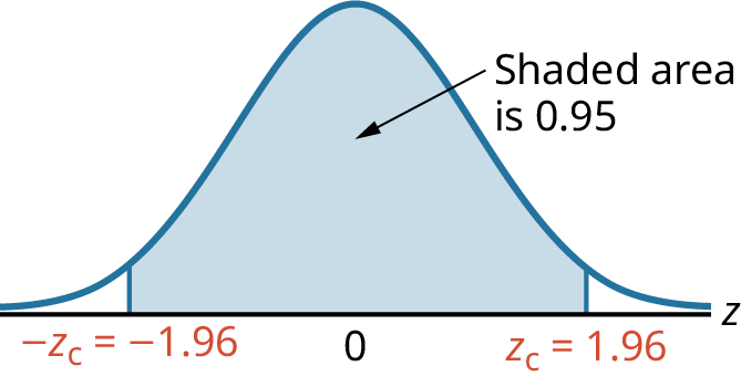
$z_{c}$ is called the critical value of the normal distribution and is calculated as the z-score, which includes the area corresponding to the confidence level between $- z_{c}$ and $+ z_{c}$ . For example, for a 95% confidence interval, the corresponding critical value is $z sub c equals 1.96$ since an area of 0.95 under the normal curve is contained between the z-scores of $minus 1.96$ and $plus 1.96$ .

$σ$ is the population standard deviation.

$n$ is the sample size.

Note: $\frac{σ}{\sqrt{n}}$ is called the standard error of the mean.

Typical values of $z_{c}$ for various confidence levels are shown in Table 4.2.

**Table 4.2**
Confidence Level	Value of $z_{c}$
80% confidence	1.280
90% confidence	1.645
95% confidence	1.960
99% confidence	2.575

Graphically, the critical values can be marked on the normal distribution curve, as shown in Figure 4.2. (See Discrete and Continuous Probability Distributions for a review of the normal distribution curve.) Figure 4.2 is an example for a 95% confidence interval where the area of 0.95 is centered as the area under the standard normal curve showing the values of $- z_{c}$ and $+ z_{c}$ . Since the standard normal curve is symmetric, and since the total area under the curve is known to be 1, the area in each of the two tails can be calculated to be 0.025. Thus, the critical value is that z-score which cuts off an area of 0.025 in the upper tail of the standard normal curve.

A standard normal curve for 95 percent confidence interval with area under the curve shaded blue. Critical values of negative z_c and z_c, labeled negative 1.96 and 1.96, respectively. — **Figure 4.2** Critical Values of z_c Marked on Standard Normal Curve for 95% Confidence Interval

Once the margin of error has been calculated, the confidence interval can be calculated as follows:

$Sample Mean \pm Margin of Error$

Note that this is the general format for constructing any confidence interval, namely the margin of error is added and subtracted to the sample statistic to generate the upper and lower bounds of the confidence interval, respectively. A sample statistic describes some aspect of the sample, such as a sample mean or sample proportion.

General Form of a Confidence Interval: $Sample Statistic \pm Margin of Error$

Example 3

A college professor collects data on the amount of time spent on homework assignments per week for a sample of 50 students in a statistics course. From the sample of 50 students, the mean amount of time spent on homework assignments per week is 12.5 hours. The population standard deviation is known to be 6.3 hours.

The professor would like to forecast the amount of time spent on homework in future semesters. Create a forecasted confidence interval using both a 90% and 95% confidence interval and provide a conclusion regarding the confidence interval. Also compare the widths of the two confidence intervals. Which confidence interval is wider?

Calculation for 90% Confidence Interval

For a 90% confidence interval, the corresponding critical value is $z sub c equals 1.645$ .

The margin of error is calculated as follows:

$E = z_{c} \frac{σ}{\sqrt{n}} = 1.645 \cdot \frac{6.3}{\sqrt{50}} = 1.47$

The 90% confidence interval is calculated as follows:

$\begin{array}{rcl} Lower Bound of the Confidence Interval & = & Point Estimate - Margin of Error \\ = & 12.5 - 1.47 = 11.03 \\ Upper Bound of the Confidence Interval & = & Point Estimate + Margin of Error \\ = & 12.5 + 1.47 = 13.97 \end{array}$

Concluding statement:

The college professor can forecast with 90% confident that the mean amount of time spent on homework assignments in a future semester is the interval from 11.03 to 13.97 hours per week.

Calculation for 95% Confidence Interval

For a 95% confidence interval, the corresponding critical value is $z sub c equals 1.960$ .

The margin of error is calculated as follows:

$E = z_{c} \frac{σ}{\sqrt{n}} = 1.960 \cdot \frac{6.3}{\sqrt{50}} = 1.75$

The 95% confidence interval is calculated as follows:

$\begin{array}{rcl} Lower Bound of the Confidence Interval & = & Point Estimate - Margin of Error \\ = & 12.5 - 1.75 = 10.75 \\ Upper Bound of the Confidence Interval & = & Point Estimate + Margin of Error \\ = & 12.5 + 1.75 = 14.25 \end{array}$

Concluding statement:

The college professor can forecast with 95% confident that the mean amount of time spent on homework assignments in a future semester is the interval from 10.75 to 14.25 hours per week.

Comparison of 90% and 95% confidence intervals:

The 90% confidence interval extends from 11.03 to 13.97.
The 95% confidence interval extends from 10.75 to 14.25.

Notice that the 95% confidence interval is wider. If the confidence level is increased, with all other parameters held constant, we should expect that the confidence interval will become wider. Another way to consider this: the wider the confidence interval, the more likely the interval is to contain the true population mean. This makes intuitive sense in that if you want to be more certain that the true value of the parameter is within an interval, then the interval needs to be wider to account for a larger range of potential values. As an analogy, consider a person trying to catch a fish. The wider the net used, the higher the probability of catching a fish.

You might notice that the sample size $n$ is located in the denominator of the formula for margin of error. This indicates that as the sample size increases, the margin of error will decrease, which will then result in a narrower confidence interval. On the other hand, as the sample size decreases, the margin of error increases and the confidence interval becomes wider.

Confidence Interval for the Mean When the Population Standard Deviation Is Unknown

A confidence interval can still be determined when the population standard deviation is unknown by calculating a sample standard deviation based on the sample data. This is actually the more common application of confidence intervals.

Here are the conditions required to use this procedure:

A random sample is selected from the population.
The sample size is at least 30, or the underlying population is known to follow a normal distribution.
The population standard deviation ( $σ$ ) is unknown; the sample standard deviation $(s)$ can be calculated.

Once these requirements are met, the margin of error (E) is calculated according to the following formula:

$E = t_{c} \frac{s}{\sqrt{n}}$

$t_{c}$ is called the critical value of the t-distribution. The t-distribution is a bell-shaped, symmetric distribution similar to the normal distribution, though the t-distribution has “thicker tails” as compared to the normal distribution. The comparison of the normal and t-distribution curves is shown in Figure 4.3.

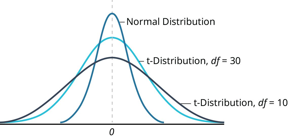
Graph showing a normal distribution curve with a peak at zero, compared to two t-distributions with degrees of freedom v=30 and v=10, both also centered at zero. — **Figure 4.3** Comparison of t-Distribution and Normal Distribution Curves

The t-distribution is actually a family of curves, determined by a parameter called degrees of freedom (df), where df is equal to $n minus 1$ . The critical value $t_{c}$ is similar to a z-score and specifies the area under the t-distribution curve corresponding to the confidence level between $- t_{c}$ and $+ t_{c}$ . Values of $t_{c}$ can be obtained using either a look-up table or technology.

For example, for a 95% confidence interval and sample size of 30, the corresponding critical value is $t sub c equals 2.045$ since an area of 0.95 under the t-distribution curve is contained between the t-scores of $minus 2.045$ and $plus 2.045$ .

$s$ is the sample standard deviation.

$n$ is the sample size.

df is degrees of freedom, where $d f = n - 1$ .

Typical values of $t_{c}$ for various confidence levels and degrees of freedom are shown in Table 4.3.

**Table 4.3**
	Confidence Level
Degrees of Freedom (df)	90% Confidence	95% Confidence	99% Confidence
1	6.314	12.706	63.657
2	2.920	4.203	9.925
3	2.353	3.182	5.841
4	2.132	2.776	4.604
5	2.015	2.571	4.032
10	1.812	2.228	3.169
15	1.753	2.131	2.947
20	1.725	2.086	2.845
25	1.708	2.060	2.787
30	1.697	2.042	2.750

Note that Python can be used to calculate these critical values. Python provides a function called t.ppf that generates the value of the t-distribution corresponding to a specified area under the t-distribution curve and specified degrees of freedom. This function is part of the scipy.stats library.

The syntax for the function is:
t.ppf(area to left, degrees of freedom)

For example, for a 95% confidence interval, there is an area of 0.95 centered under the t-distribution curve, which leaves a remaining area of 0.05 for the two tails of the distribution, which implies an area of 0.025 in each tail. To find a critical value corresponding to the upper 0.025 area, note that the area to the left of this critical value will then be 0.975.

Here is an example of Python code to generate the critical value $t_{c}$ for a 95% confidence interval and 15 degrees of freedom.

Note

# import function from scipy.stats library
from scipy.stats import t

# define parameters called area to left and degrees of freedom df
Area_to_left = 0.975
df = 15

# use t.ppf function to calculate critical values associated with t-
# use round function to round answer to 3 decimal places
round (t.ppf(Area_to_left, df), 3)

The resulting output will look like this:

2.131

Once the margin of error is calculated, the confidence interval is formed in the same way as the previous section, namely:

$\begin{array}{rcl} Lower Bound of the Confidence Interval & = & Point Estimate - Margin of Error \\ Upper Bound of the Confidence Interval & = & Point Estimate + Margin of Error \end{array}$

Example 4

A company’s human resource administrator wants to estimate the average commuting distance for all 5,000 employees at the company. Since it is impractical to collect commuting distances from all 5,000 employees, the administrator decides to sample 16 employees and collects data on commuting distance from each employee in the sample. The sample data indicates a sample mean of 15.8 miles with a standard deviation of 3.2 miles. Calculate a 99% confidence interval and provide a conclusion regarding the confidence interval.

Since the sample size is 16 employees, the degrees of freedom is one less than the sample size, which is $d f equals 15$ . For a 99% confidence interval, the corresponding critical value is $t sub c equals 2.947$ .

The margin of error is calculated as follows:

$E = t_{c} \frac{s}{\sqrt{n}} = 2.947 \cdot \frac{3.2}{\sqrt{16}} = 2.36$

The 99% confidence interval is calculated as follows:

$\begin{array}{rcl} Lower Bound of the Confidence Interval & = & Point Estimate - Margin of Error \\ = & 15.8 - 2.36 = 13.44 \\ Upper Bound of the Confidence Interval & = & Point Estimate + Margin of Error \\ = & 15.8 + 2.36 = 18.16 \end{array}$

Concluding statement:

The administrator can be 99% confident that the true population mean commuting distance for all employees is between 13.44 to 18.16 miles.

Confidence Interval for Proportions

We can also calculate a confidence interval for a population proportion based on the use of sample data. The basis for the confidence interval will be the application of a normal approximation to the binomial distribution. Recall from Discrete and Continuous Probability Distributions that a binomial distribution is a probability distribution for a discrete random variable where there are only two possible outcomes of an experiment. A proportion measures the number of successes in a sample. For example, if 10 survey respondents out of 50 indicate they are planning to travel internationally within the next 12 months, then the proportion is 10 out of 50, which is 0.2, or 20%. Note that the term success does not necessarily imply a positive outcome. For example, a researcher might be interested in the proportion of smokers among U.S. adults, and the number of smokers would be considered the number of successes.

Some terminology will be helpful:
$p$ represents the population proportion, which is typically unknown.
$p ^$ represents the sample proportion.
$x$ represents the number of successes in the sample.
$n$ represents the sample size.

Here are the requirements to use this procedure:

A random sample is selected from the population.
Verify that the normal approximation to the binomial distribution is appropriate by ensuring that both $n p ^$ and $n open parenthesis 1 minus p ^ close parenthesis$ are both at least 5, where $p ^$ represents the sample proportion.

The sample proportion $p ^$ is calculated as the number of successes divided by the sample size:

$\hat{p} = \frac{x}{n}$

When these requirements are met, the margin of error (E) for a confidence interval for proportions is calculated according to the following formula:

$E = z_{c} \sqrt{\frac{\hat{p} (1 - \hat{p})}{n}}$

Where:

$z_{c}$ is called the critical value of the normal distribution and is calculated as the z-score, which includes the area corresponding to the confidence level between $- z_{c}$ and $+ z_{c}$ .

$p ^$ represents the sample proportion.

$n$ is the sample size.

Once the margin of error is calculated, the confidence interval is formed in the same way as the previous section. In this case, the point estimate is the sample proportion $p ^$ :

$\begin{array}{rcl} Lower Bound of the Confidence Interval & = & Point Estimate - Margin of Error \\ Upper Bound of the Confidence Interval & = & Point Estimate + Margin of Error \end{array}$

Example 5

A medical researcher wants to know if there has been a statistically significant change in the proportion of smokers from five years ago, when the proportion of adult smokers in the United States was approximately 28%. The researcher selects a random sample of 1,500 adults, and of those, 360 respond that they are smokers. Calculate a 95% confidence interval for the true population proportion of adults who smoke. Also, determine if there has been a statistically significant change in the proportion of smokers as compared to five years ago.

For a 95% confidence interval, the corresponding critical value is $z sub c equals 1.960$ .

Start off by calculating the sample proportion $p ^$ :

$\hat{p} = \frac{x}{n} = \frac{360}{1,500} = 0.24$

Verify that the normal approximation to the binomial distribution is appropriate by ensuring that both $n p ^$ and $n open parenthesis 1 minus p ^ close parenthesis$ are both at least 5, where $p ^$ represents the sample proportion.

For this example, $n \hat{p} = (1,500) (0.24) = 360$ , and $n (1 - \hat{p}) = (1,500) (1 - 0.24) = 1,140$ . Both of these results are at least 5, which verifies that the normal approximation to the binomial distribution is appropriate.

The margin of error is then calculated as follows:

$E = z_{c} \sqrt{\frac{\hat{p} (1 - \hat{p})}{n}} = 1.960 \sqrt{\frac{0.24 (1 - 0.24)}{1,500}} = 0.022$

The 95% confidence interval is calculated as follows:

$\begin{array}{rcl} Lower Bound of the Confidence Interval & = & Point Estimate - Margin of Error \\ = & 0.24 - 0.022 = 0.218 \\ Upper Bound of the Confidence Interval & = & Point Estimate + Margin of Error \\ = & 0.24 + 0.022 = 0.262 \end{array}$

Concluding statement:

The researcher can be 95% confident that the true population of adult smokers in the United States is between 0.218 and 0.262, which can also be written as 21.8% to 26.2%. Since this 95% confidence interval excludes the previous value of 28% from five years ago, the researcher can state that there has been a statistically significant decrease in the proportion of smokers as compared to five years ago.

Sample Size Determination

When collecting sample data in order to construct a confidence interval for a mean or proportion, how does the researcher determine the optimal sample size? Too small of a sample size may lead to a wide confidence interval that is not very useful. Too large of a sample size can result in wasted resources if a smaller sample size would be sufficient. Sampling is covered in some depth in Handling Large Datasets. Here, we review methods to determine minimum sample size requirements when constructing confidence intervals for means or proportions. Note that the desired margin of error plays a key role in this sample size determination.

Sample Size for Confidence Interval for the Mean

When determining a confidence interval for a mean, a researcher can use the margin of error formula for the mean; solving this formula algebraically for the sample size ( $n$ ), the following minimum sample size formula can be used to determine the minimum sample size needed to achieve a certain margin of error:

Sample size formula for confidence interval for mean:

$E = z_{c} \frac{σ}{\sqrt{n}} \to n = {(\frac{z_{c} σ}{E})}^{2}$

Where:
$z_{c}$ is the critical value of the normal distribution.
$σ$ is the population standard deviation.
$E$ is the desired margin of error.

Note that for sample size calculations, sample size results are rounded up to the next higher whole number. For example, if the formula previously shown results in a sample size of 59.2, then the sample size will be rounded to 60.

Example 6

A benefits analyst is interested in a 90% confidence interval for the mean salary for chemical engineers. What sample size should the analyst use if a margin of error of $1,000 is desired? Assume a population standard deviation of $8,000.

For a 90% confidence interval, the corresponding critical value is $z sub c equals 1.645$ . The population standard deviation is given as $8,000, and the margin of error is given as $1,000.

Using the sample size formula:

$n = {(\frac{z_{c} σ}{E})}^{2} = {(\frac{1.645 \cdot 8000}{1000})}^{2} = 173.2$

Round to the next higher whole number, so the desired sample size is 174.

The analyst should target a sample size of 174 chemical engineers for a salary-related survey in order to them calculate a 90% confidence interval for the mean salary of chemical engineers.

Sample Size for Confidence interval for a Proportion

In Example 5, how would the researcher know the optimal sample size to use to collect sample data on the proportion of adults who are smokers? The margin of error formula can be used to derive the sample size for a proportion as follows:

$n = {\hat{p} (1 - \hat{p}) (\frac{z_{c}}{E})}^{2}$

Where:
$z_{c}$ is the critical value of the normal distribution.
$p ^$ is the sample proportion.
$E$ is the desired margin of error.

Notice in this formula, it’s assumed that some prior estimate for the sample proportion $p ^$ is available, perhaps from historical data or previous studies. If a prior estimate for the sample proportion is not available, then use the value of 0.5 for $p ^$ .

Example 7

Political candidate Smith is planning a survey to determine a 95% confidence interval for the proportion of voters who plan to vote for Smith. How many people should be surveyed? Assume a margin of error is 3%.

Assume there is no prior estimate for the proportion of voters who plan to vote for candidate Smith.
Assume that from prior election results, approximately 42% of people previously voted for candidate Smith.

For a 95% confidence interval, the corresponding critical value is $z sub c equals 1.960$ . The margin of error is specified as 0.03. Since a prior estimate for the sample proportion is unknown, use a value of 0.5 for $p ^$ .
Using the sample size formula:

$n = {\hat{p} (1 - \hat{p}) (\frac{z_{c}}{E})}^{2} = 0.5 (1 - 0.5) {(\frac{1.960}{0.03})}^{2} = 1,067.1$
Round to the next higher whole number, so the desired sample size is 1,068 people to be surveyed.
Since a prior estimate for the sample proportion is available, use the value of 0.42 for $p ^$ .
Using the sample size formula:

$n = {\hat{p} (1 - \hat{p}) (\frac{z_{c}}{E})}^{2} = 0.42 (1 - 0.42) {(\frac{1.960}{0.03})}^{2} = 1039.8$
Round to the next higher whole number, so the desired sample size is 1,040 people to be surveyed.
Note that having a prior estimate of the sample proportion will result in a smaller sample size requirement. This is a general conclusion, so if a researcher has a prior estimate for the population proportion, this will result in a smaller sample size requirement as compared to the situation where no prior estimate is available.

Bootstrapping Methods

In the earlier discussion of confidence intervals, certain requirements needed to be met in order to use the estimation methods. For example, when calculating the confidence interval for a mean, this requirement was indicated:

The sample size is at least 30, or the underlying population is known to follow a normal distribution.

When calculating the confidence interval for a proportion, this requirement was noted:

Verify that the normal approximation to the binomial distribution is appropriate by ensuring that both $n p ^$ and $n open parenthesis 1 minus p ^ close parenthesis$ are at least 5.

What should a researcher do when these requirements are not met? Fortunately, there is another option called “bootstrapping” that can be used to find confidence intervals when the underlying distribution is unknown or if one of the conditions is not met. This bootstrapping method involves repeatedly taking samples with replacement.

Sampling with replacement means that when a sample is selected, the sample is replaced back in the dataset before selecting the next sample. For example, a casino dealer plans to take a sample of two cards from a standard 52-card deck. If the sampling is to be done with replacement, then after selecting the sample of the first card, this card is then returned to the deck before the second card is selected. This implies that the same data value can appear multiple times in a given sample since once a data value is selected for the sample, it is replaced back in the dataset and is eligible to be selected again for the sample.

For example, a researcher who has collected 100 samples to use for inference may want to estimate a confidence interval for the population mean. The researcher can then resample, with replacement, from this limited set of 100 observations. They would repeatedly sample 100 and calculate the sample mean. These means would then represent the distribution of means (remember the discussion of sampling distribution). Typically, for bootstrapping, repeated samples are taken hundreds or thousands of times and then the sample mean is calculated for each sample.

The term “bootstrapping” comes from the old saying “pull yourself up by your bootstraps” to imply a task that was accomplished without any outside help. In the statistical sense, bootstrapping refers to the ability to estimate parameters based solely on one sample of data from the population without any other assumptions.

The bootstrapping method is considered a nonparametric method since the technique makes no assumptions about the probability distribution from which the data are sampled. (Parametric methods, by contrast, assume a specific form for the underlying distribution and require estimating parameters.)

Since bootstrapping requires a large number of repeated samples, software (such as Excel, Python, or R) is often used to automate the repetitive sampling procedures and construct the confidence intervals.

The bootstrapping procedure for confidence interval estimation for a mean or proportion is as follows:

Start out with a random sample of size $n$ . Collect many random bootstrap samples of size $n$ —for example, hundreds or thousands of such samples. Keep in mind that the sampling is done with replacement.
For each sample, calculate the sample statistic, which is the sample mean $\bar{x}$ or the sample proportion $p ^$ .
Rank order the sample statistics from smallest to largest.
For a 95% confidence interval, find the percentiles P_2.5 and P_97.5 in the ranked data. These values establish the 95% confidence interval.
For a 90% confidence interval, find the percentiles P₅ and P₉₅. These values establish the 90% confidence interval.

Example 8

A college administrator is developing new marketing materials to increase enrollment at the college, and the administrator is interested in a 90% confidence interval for the mean age of students attending the college.

The administrator believes the underlying distribution of ages is skewed (does not follow a normal distribution), so a bootstrapping method will be used to construct the confidence interval. The administrator selects a random sample of 20 students and records their ages as shown in Table 4.4. Use the bootstrapping method to construct the 90% confidence interval by taking repeated samples of size 10.

**Table 4.4**
Student ID	Student Age
001	22
002	24
003	21
004	34
005	29
006	23
007	21
008	20
009	19
010	21
011	25
012	28
013	22
014	37
015	24
016	31
017	23
018	19
019	26
020	20

For the bootstrapping process, we will form samples of size 10 for convenience. Note that the sampling is with replacement, so once an age is selected, the age is returned back to the dataset and then that particular age might be selected again as part of the sample.

Imagine forming hundreds or thousands of such samples, each of sample size 10. For each one of these samples, calculate the sample mean (see column labeled “Sample Means”).

In the example shown in Figure 4.4, only 20 samples are taken for space considerations since showing the results of thousands of samples is not practical for this text. However, typically a bootstrapping process involves many such samples—on the order of thousands of samples—made possible by using software (such as Excel, Python, or R).

Figure 4.4 Bootstrap Samples and Corresponding Sample Means

Next, sort the sample means from smallest to largest (see column labeled “Sorted Sample Means”).

The last step is to calculate the 90% confidence interval based on these sorted sample means. For a 90% confidence interval, find the percentiles P₅ and P₉₅. These values establish the 90% confidence interval.

To find the 5th percentile (P₅), multiply the percentile (5%) times the number of data values, which is 20. The result is 1, so to find the 5th percentile, add the first and second data values together and divide by 2. For this example, add 21.9 to 22.2 and divide by 2. The result is 22.05.

To find the 95th percentile (P₉₅), multiply the percentile (95%) times the number of data values, which is 20. The result is 19, so to find the 95th percentile, add the 19th and 20th data values together and divide by 2. For this example, add 28.5 to 28.6 and divide by 2. The result is 28.6.

Based on the bootstrapping method, the 90% confidence interval is (22.05, 28.6).

Python provides a function called bootstrap as part of the scipy.stats library to automate this bootstrapping process.

Within the bootstrapfunction, the user can specify the number of resamples to be performed as part of the bootstrapping process. In this example, we will use 50,000 samples by way of the $n$ _resample parameter.

Note

from scipy.stats import bootstrap
import numpy as np

#define random sample of ages
ages = [22, 23, 25, 31, 24, 21, 28, 23, 21, 20, 22, 19, 34, 19, 37, 26, 29, 21, 24, 20]

#convert ages to sequence
ages = (ages,)

#use bootstrap function for confidence interval for the mean
conf_interval = bootstrap(ages, np.mean, confidence_level=0.95,
                         random_state=1, n_resamples = 50000, method='percentile')

#print the confidence interval
print(conf_interval.confidence_interval)

The resulting output will look like this:

ConfidenceInterval(low=22.45, high=26.7)

Using 50,000 bootstrapped samples, a 95% confidence interval is generated as (22.45, 26.7).

Using Python to Calculate Confidence Intervals

When calculating confidence intervals, data scientists typically make use of technology to help streamline and automate the analysis. Python provides built-in functions for confidence interval calculations, and several examples are shown in Table 4.5. Students are encouraged to try examples themselves and experiment to use Python to assist with these calculations.

Table 4.5 provides a summary of various functions available within the SciPy library for confidence interval calculations:

**Table 4.5**
Usage	Python Function Name	Syntax
Calculate confidence interval for the mean when population standard deviation is known, given sample mean, population standard deviation, and sample size (uses normal distribution).	`norm.interval`	`norm.interval(conf_level, sample_mean,standard_dev/sqrt (n))`
Calculate confidence interval for the mean when population standard deviation is unknown, given sample mean, sample standard deviation, and sample size (uses t-distribution).	`t.interval`	`t.interval(conf_level, degrees_freedom, sample_mean,standard_dev/sqrt (n))`
Calculate confidence interval for a proportion (uses normal distribution).	`proportion_confint`	`proportion_confint(success, sample_size, 1 – confidence_level)`

Example 9

Repeat Example 3 to calculate a 90% confidence interval, but use Python functions to calculate the confidence interval.

Recall from Example 3, the sample mean is 12.5 hours with a population standard deviation of 6.3 hours. The sample size is 50 students, and we are interested in calculating a 90% confidence interval.

Use the Python function norm.interval as shown:

Note

import scipy.stats as stats
import numpy as np
import math

# Enter sample mean, population standard deviation and sample size
sample_mean = 12.5
population_standard_deviation = 6.3
sample_size = 50 

# Confidence level 
confidence_level = 0.90

# standard error
standard_error = population_standard_deviation / math.sqrt(sample_size)

# Calculate confidence interval using norm.interval function
stats.norm.interval(confidence_level, sample_mean, standard_error)

The resulting output will look like this:

(11.03451018636739, 13.965489813632608)

Example 10

Repeat Example 4 to calculate a 99% confidence interval, but use Python functions to calculate the confidence interval.

Recall from Example 4, the sample mean is 15.8 miles with a standard deviation of 3.2 miles. The sample size is 26 employees, and we are interested in calculating a 99% confidence interval.

Use the Python function t.interval as shown:

Note

# Enter sample mean, sample standard deviation, and sample size
sample_mean = 15.8
sample_standard_deviation = 3.2
sample_size = 26 

# Degrees of freedom (sample size - 1)
degrees_of_freedom = sample_size - 1

# Confidence level 
confidence_level = 0.99

# standard error
standard_error = sample_standard_deviation / math.sqrt(sample_size)

# Calculate confidence interval using t.interval function
t.interval(confidence_level, degrees_of_freedom, sample_mean, standard_error)

The resulting output will look like this:

(14.050684356083625, 17.549315643916376)

Student ID	Student Age
001	22
002	24
003	21
004	34
005	29
006	23
007	21
008	20
009	19
010	21
011	25
012	28
013	22
014	37
015	24
016	31
017	23
018	19
019	26
020	20

Student ID	Student Age
001	22
002	24
003	21
004	34
005	29
006	23
007	21
008	20
009	19
010	21
011	25
012	28
013	22
014	37
015	24
016	31
017	23
018	19
019	26
020	20

Student ID	Student Age
001	22
002	24
003	21
004	34
005	29
006	23
007	21
008	20
009	19
010	21
011	25
012	28
013	22
014	37
015	24
016	31
017	23
018	19
019	26
020	20