
6.6 Hamiltonian Circuits and the Traveling Salesman Problem
In the last section, we considered optimizing a walking route for a postal carrier. How is this different than the requirements of a package delivery driver? While the postal carrier needed to walk down every street (edge) to deliver the mail, the package delivery driver instead needs to visit every one of a set of delivery locations. Instead of looking for a circuit that covers every edge once, the package deliverer is interested in a circuit that visits every vertex once.
Hamiltonian circuits are named for William Rowan Hamilton who studied them in the 1800’s.
Unlike with Euler circuits, there is no nice theorem that allows us to instantly determine whether or not a Hamiltonian circuit exists for all graphs.[1]
With Hamiltonian circuits, our focus will not be on existence, but on the question of optimization; given a graph where the edges have weights, can we find the optimal Hamiltonian circuit; the one with lowest total weight.
This problem is called the Traveling salesman problem (TSP) because the question can be framed like this: Suppose a salesman needs to give sales pitches in four cities. He looks up the airfares between each city, and puts the costs in a graph. In what order should he travel to visit each city once then return home with the lowest cost?
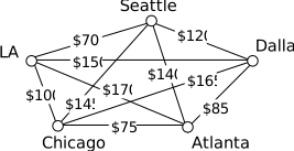
To answer this question of how to find the lowest cost Hamiltonian circuit, we will consider some possible approaches. The first option that might come to mind is to just try all different possible circuits.
The Brute force algorithm is optimal; it will always produce the Hamiltonian circuit with minimum weight. Is it efficient? To answer that question, we need to consider how many Hamiltonian circuits a graph could have. For simplicity, let’s look at the worst-case possibility, where every vertex is connected to every other vertex. This is called a complete graph.
Suppose we had a complete graph with five vertices like the air travel graph above. From Seattle there are four cities we can visit first. From each of those, there are three choices. From each of those cities, there are two possible cities to visit next. There is then only one choice for the last city before returning home.
This can be shown visually:
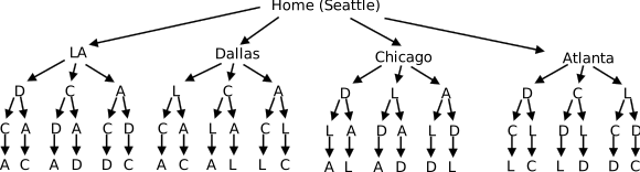
Counting the number of routes, we can see there are routes. For six cities there would be routes.
While this is a lot, it doesn’t seem unreasonably huge. But consider what happens as the number of cities increase:
| Citices | Unique Hamiltonian Circuits |
|---|---|
| 9 | 8 ! / 2 = 20,160 |
| 10 | 9 ! / 2 = 181,440 |
| 11 | 10 ! / 2 = 1,814,400 |
| 15 | 14 ! / 2 = 43,589,145,600 |
| 20 | 19 ! / 2=60,822,550,204,416,000 |
As you can see the number of circuits is growing extremely quickly. If a computer looked at one billion circuits a second, it would still take almost two years to examine all the possible circuits with only 20 cities! Certainly Brute Force is not an efficient algorithm.
Unfortunately, no one has yet found an efficient and optimal algorithm to solve the TSP, and it is very unlikely anyone ever will. Since it is not practical to use brute force to solve the problem, we turn instead to heuristic algorithms; efficient algorithms that give approximate solutions. In other words, heuristic algorithms are fast, but may or may not produce the optimal circuit.
We ended up finding the worst circuit in the graph! What happened? Unfortunately, while it is very easy to implement, the NNA is a greedy algorithm, meaning it only looks at the immediate decision without considering the consequences in the future. In this case, following the edge AD forced us to use the very expensive edge BC later.
# Ch 6.6 - four algorithms, one Travelling Salesman graph. Watch a heuristic lose.
# TRY IT: drop the expensive edge B-C from 13 to 3 and re-run. Does greedy
# nearest-neighbour still walk into the trap?
from itertools import permutations
import matplotlib.pyplot as plt

W = {("A", "B"): 4, ("A", "C"): 2, ("A", "D"): 1,
     ("B", "C"): 13, ("B", "D"): 9, ("C", "D"): 8}
G = {}
for (u, v), w in W.items():
    G.setdefault(u, {})[v] = w
    G.setdefault(v, {})[u] = w
V = sorted(G)
cost = lambda tour: sum(G[a][b] for a, b in zip(tour, tour[1:]))

def nearest_neighbour(start):
    tour, left = [start], set(V) - {start}
    while left:
        nxt = min(left, key=lambda v: G[tour[-1]][v])
        tour.append(nxt)
        left.discard(nxt)
    return tour + [start]           # greedy: never looks past the next hop

def sorted_edges():
    deg, parent, keep = {v: 0 for v in V}, {v: v for v in V}, []
    def find(v):
        while parent[v] != v:
            v = parent[v]
        return v
    for (u, v), w in sorted(W.items(), key=lambda kv: kv[1]):
        if deg[u] == 2 or deg[v] == 2:                    # would make a degree 3
            continue
        if find(u) == find(v) and len(keep) < len(V) - 1:  # closes a short circuit
            continue
        parent[find(u)] = find(v)
        deg[u] += 1
        deg[v] += 1
        keep.append((u, v))
    tour, cur, used = [V[0]], V[0], set()
    while len(tour) <= len(V):
        e = next(x for x in keep if cur in x and x not in used)
        used.add(e)
        cur = e[0] if e[1] == cur else e[1]
        tour.append(cur)
    return tour

best = min(([V[0]] + list(p) + [V[0]] for p in permutations(V[1:])), key=cost)
runs = ([("brute force (all circuits)", best)]
        + [(f"nearest neighbour from {s}", nearest_neighbour(s)) for s in V]
        + [("repeated nearest neighbour", min((nearest_neighbour(s) for s in V), key=cost)),
           ("sorted edges / cheapest link", sorted_edges())])
for label, tour in runs:
    gap = cost(tour) - cost(best)
    print(f"{label:<30} {''.join(tour):<7} weight {cost(tour):>3}"
          + ("  <-- optimal" if gap == 0 else f"  {gap} worse than optimal"))

pos = {"A": (0, 1), "B": (1, 1), "C": (0, 0), "D": (1, 0)}
fig, axes = plt.subplots(1, 2, figsize=(9, 4.2))
for ax, tour in zip(axes, [best, nearest_neighbour("A")]):
    for (u, v), w in W.items():
        (x0, y0), (x1, y1) = pos[u], pos[v]
        ax.plot([x0, x1], [y0, y1], color="0.85", zorder=1)
        ax.text(x0 + 0.35 * (x1 - x0), y0 + 0.35 * (y1 - y0), str(w),
                color="0.35", ha="center", va="center", fontsize=9)
    for a, b in zip(tour, tour[1:]):
        ax.plot([pos[a][0], pos[b][0]], [pos[a][1], pos[b][1]], "tab:red", lw=2.5, zorder=2)
    for v, (x, y) in pos.items():
        ax.plot(x, y, "o", ms=24, color="white", mec="black", zorder=3)
        ax.text(x, y, v, ha="center", va="center", zorder=4)
    ax.set_title(f"{''.join(tour)}   weight {cost(tour)}", fontsize=11); ax.axis("off")
plt.suptitle("left: brute force optimum      right: nearest neighbour from A")
plt.tight_layout(); plt.show()Going back to our first example, how could we improve the outcome? One option would be to redo the nearest neighbor algorithm with a different starting point to see if the result changed. Since nearest neighbor is so fast, doing it several times isn’t a big deal.
While certainly better than the basic NNA, unfortunately, the RNNA is still greedy and will produce very bad results for some graphs. As an alternative, our next approach will step back and look at the “big picture” – it will select first the edges that are shortest, and then fill in the gaps.
While the Sorted Edge algorithm overcomes some of the shortcomings of NNA, it is still only a heuristic algorithm, and does not guarantee the optimal circuit.
[1] There are some theorems that can be used in specific circumstances, such as Dirac’s theorem, which says that a Hamiltonian circuit must exist on a graph with n vertices if each vertex has degree n/2 or greater.
Adapted from Math in Society by David Lippman, hosted on LibreTexts (math.libretexts.org) and licensed under CC BY-SA 3.0. Changes were made. License: CC-BY-SA-3.0.